
This publication was made possible through the cooperation of Biblioteca Italia, a Giovanni Agnelli Foundation program for the diffusion of Italian culture.
This fifth edition first published in English 2012
English translation © 2012 John Wiley & Sons, Ltd
Originally published in Italian as Storia minima della populazione del mondo © 2011 Massimo Livi-Bacci
English edition history: Blackwell Publishers Ltd (1e, 1992; 2e, 1997 and 3e, 2001);
Blackwell Publishing Ltd (4e, 2007)
Wiley-Blackwell is an imprint of John Wiley & Sons, formed by the merger of Wiley’s global Scientific, Technical and Medical business with Blackwell Publishing.
Registered Office
John Wiley & Sons, Ltd, The Atrium, Southern Gate, Chichester, West Sussex, PO19 8SQ, UK
Editorial Offices
350 Main Street, Malden, MA 02148–5020, USA
9600 Garsington Road, Oxford, OX4 2DQ, UK
The Atrium, Southern Gate, Chichester, West Sussex, PO19 8SQ, UK
For details of our global editorial offices, for customer services, and for information about how to apply for permission to reuse the copyright material in this book please see our website at .
The right of Massimo Livi-Bacci to be identified as the author of this work has been asserted in accordance with the UK Copyright, Designs and Patents Act 1988.
All rights reserved. No part of this publication may be reproduced, stored in a retrieval system, or transmitted, in any form or by any means, electronic, mechanical, photocopying, recording or otherwise, except as permitted by the UK Copyright, Designs and Patents Act 1988, without the prior permission of the publisher.
Wiley also publishes its books in a variety of electronic formats. Some content that appears in print may not be available in electronic books.
Designations used by companies to distinguish their products are often claimed as trademarks. All brand names and product names used in this book are trade names, service marks, trademarks or registered trademarks of their respective owners. The publisher is not associated with any product or vendor mentioned in this book. This publication is designed to provide accurate and authoritative information in regard to the subject matter covered. It is sold on the understanding that the publisher is not engaged in rendering professional services. If professional advice or other expert assistance is required, the services of a competent professional should be sought.
Library of Congress Cataloging-in-Publication Data
Livi-Bacci, Massimo.
[Storia minima della popolazione del mondo. English]
A concise history of world population / Massimo Livi-Bacci. – 5th ed.
p. cm.
“Originally published in Italian as Storia minima della populazione del mondo.”
Includes bibliographical references and index.
ISBN 978-0-470-67320-1 (pbk.)
1. Population–History. I. Title.
HB871.L56513 2012
304.6–dc23
2011043342
A catalogue record for this book is available from the British Library.
Contents
List of Figures
| r strategy and K strategy | |
| The length of an organism at the time of reproduction in relation to the generation time, plotted on a logarithmic scale | |
| Growth of the French Canadian population (seventeenth century): pioneers and their children | |
| Effect on the average number of children per woman of maximum variations of the components of fertility above and below the standard | |
| Fertility models | |
| Survival curves for three female populations characterized by low, medium, and high life expectancy at birth | |
| Survival models | |
| Relationship between the average number of children per woman (TFR) and life expectancy (e0) in historical and present-day populations | |
| Relationship between rainfall and primary productivity for world biomes | |
| Relationship between annual precipitation and population density (Australian Aborigines) | |
| Cycles of demographic growth | |
| Failure and success of individual populations – a model | |
| Presumed demographic effects accompanying the transition from hunting and gathering to agriculture | |
| Spread of the plague in Europe, 1347–53 | |
| The Malthusian system of positive and preventive checks during phases of demographic expansion and decline | |
| Sienese death and grain-price indices (sixteenth and seventeenth centuries) | |
| Population and grain prices in Europe (1200–1800; 1721–45 = 100) | |
| Population and real wages in England (1551–1851) | |
| Real wages, fertility (TFR), and life expectancy (e0) in England (1551–1801) | |
| Population and agricultural intensification | |
| The strategic space of growth for 17 European countries (nineteenth through twentieth centuries) | |
| Demographic transition model | |
| Attenuation of mortality swings in Sweden (1735–1920) | |
| Relationship between real GDP per capita and life expectancy (e0) for 16 industrialized countries (1870, 1913, 1950, 1980, 2000) | |
| Relationship between average age at marriage and proportion of women married at the end of the reproductive period for several countries; generations born toward the end of the nineteenth century | |
| Relationship between general fertility (If), legitimate fertility (Ig), and proportion married (Im) in 16 European countries (1870, 1900, 1930, 1960) | |
| Distribution by decade of number of provinces of Europe experiencing 10 percent decline in legitimate fertility (Ig) | |
| Relationship between real GDP per capita and children per woman (TFR) in 16 industrialized countries (1870, 1913, 1950, 1980, 2000) | |
| Emigration and natural growth for continental Europe | |
| Ratio of those employed in manufacturing industries to those engaged in agriculture (1870–1987): (a) UK, Belgium, Germany, France, Italy; (b) Spain, Denmark, Netherlands, Sweden, Switzerland | |
| Relation between life expectancy (e0) and children per woman (TFR) in 16 European countries (1870, 1913, 1950, 1980, 2000) | |
| Annual rate of increase in population and per capita GDP for 16 industrialized countries (1870–2000) | |
| Changes in the increase in population compared with changes in GDP, total and per capita, 1929 prices, overlapping decades, United States (1870–1955) | |
| Comparison of demographic transitions: rates of increase for poor and rich populations (1700–2000) | |
| Relationship between life expectancy (e0) and average number of children per woman (TFR) for 28 large less-developed countries (1950–5, 1980–5, and 2005–10) | |
| Relationship between percentage of the population served by a sewage system and infant and child mortality in 53 less-developed countries (2000) | |
| Per capita GDP and life expectancy (e0) in 28 less-developed countries (1950–5, 1980–5, and 2000–5) | |
| Mortality in the most malarial (Anuradhapura) and least malarial (Kalutara) zones of Sri Lanka (1930–60) | |
| Model of the contributions of various factors in reducing fertility from natural to replacement levels | |
| Per capita GDP and average number of children per woman (TFR) in 28 large less-developed countries (1950–5, 1980–5, and 2000–5) | |
| Absolute decline in total fertility rate (1960–5 to 1990), by level of development in 1985 and average program effort level in 1982–9 | |
| Relationship between the average number of children per woman (TFR), wanted and unwanted fertility, and contraception for 40 populations (2005–9) | |
| Age structure in: (a) China (1950 and 2025); (b) India (1950 and 2025) | |
| Annual percentage increase in per capita GDP and population in 28 major less-developed countries (1950–2000) | |
| Past and future labor-force growth in: (a) Asia; (b) sub-Saharan Africa | |
| Diffusion of AIDS during the 1970s and 1980s | |
| Per capita expenditure on health (international$) and life expectancy at birth (2002) | |
| Possible modes of approach of a population to its carrying capacity | |
| Food price index (1990 = 100), 1961–2010 | |
| Composite resources price index at constant prices, 1900–2000 | |
| Cereal production, fertilizer inputs, land cultivated (1961 = 100), 1960–2010 | |
| Rural and urban world populations (1950–2025) | |
| Population density and the proportion of built-up land for residential, industrial, and commercial purposes, Europe, 2009 |
List of Tables
| Estimated population density and size for a catchment territory of 314 km2 in different world biomes | |
| Population, total births, and years lived (10,000 BC to AD 2000) | |
| Continental populations (400 BC to AD 2000, millions) | |
| Population of central Mexico (1532–1608) | |
| Slaves taken to America (1500–1800) and population of African origin in America (1800) | |
| Comparison of the demographic behavior of French Canadian pioneers and the contemporary French population | |
| French Canadian immigration and population (1608–1949) | |
| Populations of Ireland and Japan (seventeenth–nineteenth centuries) | |
| Growth of selected European populations (1600–1850) | |
| Beginning, end, duration, and “multiplier” of the demographic transition for several countries | |
| Maximum and minimum death rates (per 1,000) in France and Sweden (eighteenth–twentieth centuries) | |
| Life expectancy in several western countries (1750–2009) | |
| Life expectancy gains in England (1871–1951) and Italy (1881–1951), broken down by contributing causes of death | |
| Average number of children per woman (TFR) for several generations in western countries (1750–1965) | |
| The results of the transition: demographic indices for Italy (1881 and 1981) | |
| Population, number of employed, production, and productivity in the UK (1785–2000) | |
| Population, GDP, and productivity in 16 more-developed countries (1870 and 2000) | |
| World population, rich and poor countries (1900–2010) | |
| Demographic indicators of world population (1950–2010) | |
| Infant and child mortality and health indices (2005–8) | |
| Estimates of the burden of disease (2004) | |
| Demographic indices for India and China (1950–2010) | |
| Gross internal investments and population of working age (2009–10) | |
| World and continental populations (1950–2050) according to UN estimates and projections | |
| The 10 most populous countries in the world (1950, 2000, 2050, and 2100) | |
| Population of world regions in 2000 and 2100, and the contribution to growth of migration, fertility, mortality, and momentum | |
| Net migration of world regions, by decade, 1950–2010 | |
| World migrant stock, 1960–2010 | |
| The HIV/AIDS epidemic at the end of 2008 |
Preface
Why is the present population of the world seven billion and not several orders of magnitude greater or smaller? For thousands of years prior to the invention of agriculture the human species must have numbered a thousandth part of what it does today; and there are those who maintain that our planet, given the available resources, could comfortably accommodate a population ten times larger than it does at present. What are the factors that through the ages determine demographic growth? How is the difficult balance with resources and environment maintained? These are fairly old questions, confronted for the first time in a modern form by Malthus, who, not by accident, inspired the work of Darwin.
In the pages of this “concise history” I intend to address these fundamental questions, discussing the underlying suppositions, the proposed solutions, the points already clarified, and those still requiring investigation. The reader will find here a general discussion of demographic development and, I hope, a guide to understanding the mechanisms which through the ages have determined population growth, stagnation, or decline.
Since the invention of fire the human species has sought to modify the environment and enrich the resources it provides. In the very long run (millennia), humanity has grown numerically in relative harmony with available resources. Certainly the system of hunting and gathering could not have allowed the survival of many more than several million people, just as the European system of agriculture could only with great difficulty have supported more than the hundred million inhabitants who lived on the continent prior to the Industrial Revolution. However, in shorter spans of time (centuries or generations) this equilibrium is not so obvious, for two fundamental reasons. The first is the recurrent action of catastrophic events – epidemics, climatic or natural disasters – which alter radically one term of the population–resources equation. The second lies in the fact that the demographic mechanisms that determine reproductive intensity, and so demographic growth, change slowly and do not “adapt” easily to rapidly evolving environmental conditions. It is frequently claimed that the human species is equipped with “self-regulating” mechanisms that allow for the speedy reestablishment of the balance between numbers and resources. However, this is only partially true, as these mechanisms – when they do work – are imperfect (and of varying efficiency from population to population and from one age to another), so much so that entire populations have disappeared – a clear sign of the failure of all attempts at regulation.
In the following pages I devote a great deal of attention to the functioning, in various contexts and periods, of the mechanisms that determine the always precarious balance between population and resources. In order to do this I have had to enlarge my plan of attack to include problems and topics – from biology to economics – rarely touched upon in demographic works, and so have been haunted by the constant fear of losing the depth of this study for the breadth of its extension. This is a calculated and consciously accepted risk. Given the frequent setbacks suffered by attempts at interdisciplinarity, the temptation to take shelter within safe disciplinary boundaries is great; but problems remain complex and in order to resolve them it is not sufficient that they be individually identified and isolated. Now and then it is worth making an attempt at reconstruction.
Note
Throughout the text I use US billion to equal 1,000,000,000.
1 Humans and Animals
Throughout human history population has been synonymous with prosperity, stability, and security. A valley or plain teeming with houses, farms, and villages has always been a sign of well-being. Traveling from Verona to Vicenza, Goethe remarked with pleasure: “One sees a continuous range of foothills… dotted with villages, castles and isolated houses … we drove on a wide, straight and well-kept road through fertile fields … The road is much used and by every sort of person.” The effects of a long history of good government were evident, much as in the ordered Sienese fourteenth-century landscapes of the Lorenzetti brothers. Similarly, Cortés was unable to restrain his enthusiasm when he gazed over the valley of Mexico and saw the lagoons bordered by villages and trafficked by canoes, the great city, and the market (in a square more than double the size of the entire city of Salamanca) that “accommodated every day more than sixty thousand individuals who bought and sold every imaginable sort of merchandise.”
This should come as no surprise. A densely populated region is implicit proof of a stable social order, of nonprecarious human relations, and of well-utilized natural resources. Only a large population can mobilize the human resources necessary to build houses, cities, roads, bridges, ports, and canals. If anything, it is abandonment and desertion rather than abundant population that has historically dismayed the traveler.
Population, then, might be seen as a crude index of prosperity. The million inhabitants of the Paleolithic Age, the 10 million of the Neolithic Age, the 100 million of the Bronze Age, the billion of the Industrial Revolution, or the 10 billion that we may attain at the end of the twenty-first century certainly represent more than simple demographic growth. Even these few figures tell us that demographic growth has not been uniform over time. Periods of expansion have alternated with others of stagnation and even decline; and the interpretation of these, even for relatively recent historical periods, is not an easy task. We must answer questions that are as straightforward in appearance as they are complex in substance: Why are we 7 billion today and not more or less, say 100 billion or 100 million? Why has demographic growth, from prehistoric times to the present, followed a particular path rather than any of numerous other possibilities? These questions are difficult but worth considering, since the numerical progress of population has been, if not dictated, at least constrained by many forces and obstacles which have determined the general direction of that path. To begin with, we can categorize these forces and obstacles as biological and environmental. The former are linked to the laws of mortality and reproduction which determine the rate of demographic growth; the latter determine the resistance which these laws encounter and further regulate the rate of growth. Moreover, biological and environmental factors affect one another reciprocally and so are not independent of one another.
Every living collectivity develops particular strategies of survival and reproduction which translate into potential and effective growth rates of varying velocity. A brief analysis of these strategies will serve as the best introduction to consideration of the specific case of the human species. Biologists have identified two large categories of vital strategies, called r and K, which actually represent simplifications of a continuum. Insects, fish, and some small mammals practice an r-strategy: these organisms live in generally unstable environments and take advantage of favorable periods (annually or seasonally) to reproduce prolifically, even though the probability of offspring survival is small. It is just because of this environmental instability, however, that they must depend upon large numbers, because “life is a lottery and it makes sense simply to buy many tickets.” r-strategy organisms go through many violent cycles with phases of rapid increase and decrease.
A much different strategy is that practiced by K-type organisms – mammals, particularly medium and large ones, and some birds – who colonize relatively stable environments, albeit populated with competitors, predators, and parasites. K-strategy organisms are forced by selective and environmental pressure to compete for survival, which in turn requires considerable investment of time and energy for the raising of offspring. This investment is only possible if the number of offspring is small.
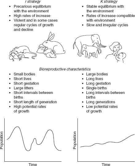
r and K strategies characterize two well-differentiated groups of organisms (). The first are suited to small animals having a short life span, minimal intervals between generations, brief gestation periods, short intervals between births, and large litters. K strategies, on the other hand, are associated with larger animals, long life spans, long intervals between generations and between births, and single births.
r strategy and K strategy
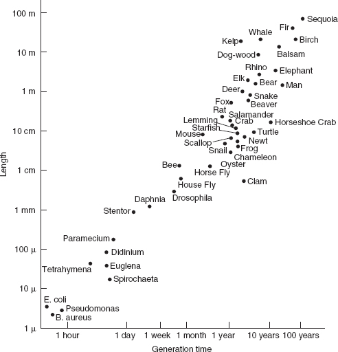
records the relation between body size (length) and the interval between successive generations for a wide array of living organisms: as the first increases, so does the second. It can also be demonstrated that the rate of growth of various species (limiting ourselves to mammals) varies more or less inversely with the length of generation and so with body size. At an admittedly macroscopic level of generalization, the lower potential for demographic growth of the larger animals can be linked to their lower vulnerability to environmental fluctuations, and this, too, is related to their larger body size. Because their life is not a lottery and their chances of survival are better, the larger animals do not need to entrust the perpetuation of the species to high levels of reproduction. The latter, in fact, would detract from those investments of protection and care required to ensure the offspring’s reduced vulnerability and keep mortality low.
The length of an organism at the time of reproduction in relation to the generation time, plotted on a logarithmic scale
Source: J.T. Bonner, Size and Cycle: An Essay on the Structure of Biology (Princeton University Press, Princeton, 1965), p.17. © 1965 Princeton University Press, 1993 renewed PUP. Reprinted by Permission of Princeton University Press.
These ideas have been well known at least since the time of Darwin and Wallace, founders of the theory of natural selection. Nonetheless, they provide a useful introduction to discussion of the factors of human increase. Our species obviously practices a K strategy, in that it has successfully controlled the fluctuating environment and invests heavily in the raising of its young.
Two principles will be particularly helpful for the purpose of confronting the arguments of the following pages. The first concerns the relation between population and environment; this should be understood broadly to include all the factors – physical environment, climate, availability of food, and so on – that determine survival. The second concerns the relation between reproduction and mortality insofar as the latter is a function of parental investment, which in turn relates inversely to reproductive intensity.
2 Divide and Multiply
Many animal species are subject to rapid and violent cycles which increase or decrease their numbers by factors of 100, 1,000, 10,000, or even more in a brief period. The four-year cycle of the Scandinavian lemming is well known, as are those of the Canadian predators (10 years) and many infesting insects of temperate woods and forests (4–12 years). In Australia, “in certain years the introduced domestic mouse multiplies enormously. The mice swarm in crops and haystacks, and literal bucketfuls can be caught in a single night. Hawks, owls and cats flourish at their expense … but all these enemies have little effect in reducing the numbers. As a rule the plague ends rather suddenly. A few dead mice are found on the ground and the numbers dwindle rapidly to, or below, normal.” Other species maintain an equilibrium. Gilbert White observed two centuries ago that eight pairs of swallows flew round the belfry of the church in the village of Selborne, just as is the case today. There are, then, both populations in rapid growth or decline and populations that are more or less stable.
The human species varies relatively slowly in time. Nonetheless, as we shall see below, long cycles of growth do alternate with others of decline, and the latter have even led to extinction for certain groups. For example, the population of Mesoamerica was reduced to a fraction of its original size during the century that followed the Spanish conquest (initiated at the beginning of the sixteenth century), while that of the conquering Spaniards grew by half. Other populations have disappeared entirely or almost entirely – the population of Santo Domingo after the landing of Columbus, or that of Tasmania following contact with the first explorers and settlers – while at the same time others nearby have continued to increase and prosper. In more recent times, the population of England and Wales multiplied sixfold between 1750 and 1900, while that of France in the same period increased by barely 50 percent. According to probable projections, the population of the Democratic Republic of Congo will multiply tenfold between 1950 and 2040, while in the meantime that of Germany will have increased by only 15 percent.
These few examples should suffice to demonstrate at what different rates the human species can grow even in similar situations (France and England) and over long periods. It should also be clear that here lies the heart of demography as a science: to measure growth, analyze mechanisms, and understand causes.
Population growth (whether positive or negative, rapid or slow) can be described by a simple calculation. In any interval of time a population (P) varies numerically as a result of renewal or arrivals (births B and immigration I) and elimination or departures (deaths D and emigration E). Leaving aside migration (considering the population “closed,” as is that of the entire planet), the change in population dP in any interval of time t – by convention and for convenience demographers use years – is given by the following:

and so the rate of growth r (where r = dP/P) will be equal to the difference between the birth rate b (where b = B/P) and the death rate d (where d = D/P):

The range of variation of the birth and death rates is fairly wide. Minimum values are 5 to 10 per thousand (possible today with mortality and fertility under control) and a maximum 40 to 50 per thousand. As mortality and fertility are not independent, it is unlikely that opposite extremes should coexist. Over long periods growth rates vary in practice between −1 and 3 percent per year.
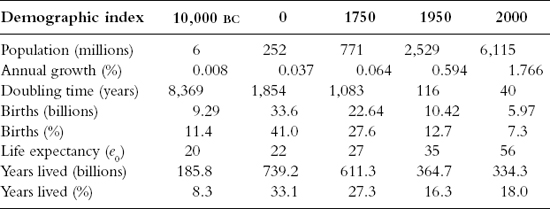
For most of human history fertility and mortality must have remained in virtual equilibrium, as the rate of population growth was very low. If we accept the estimates of 252 million for the world population at the beginning of the present era (AD 0) and 771 million in 1750 (), at the beginning of the Industrial Revolution, then we can calculate the average annual growth rate for the period as 0.06 percent. If we imagine that mortality averaged 40 per thousand, then fertility must have been 40.6 per thousand, just 1.5 percent greater than mortality. Since the 1960s the situation has been quite different, as fertility has exceeded mortality by 200 percent.
Population, total births, and years lived (10,000 BC to AD 2000)
Fertility and mortality rates are numerical calculations with little in the way of conceptual content, and as such are not well adapted to the description of the phenomena of reproduction and survival on which demographic growth depends.
3 Jacopo Bichi and Domenica Del Buono, Jean Guyon and Mathurine Robin
Jacopo Bichi was a humble sharecropper from Fiesole (near Florence). On November 12, 1667 he married Domenica Del Buono. Their marriage, although soon ended by the death of Jacopo, nonetheless produced three children: Andrea, Filippo, and Maria Maddalena. The latter died when only a few months old, but Andrea and Filippo survived and married. In a sense, Jacopo and Domenica paid off their demographic debt: the care received from their parents, and their own resistance and luck, succeeded in bringing them to reproductive age. They in turn bore and raised two children who also arrived at the same stage of maturity (reproductive age and marriage) and who, in a sense, replaced them exactly in the generational chain of life. Continuing the story of this family, Andrea married Caterina Fossi, and together they had four children, two of whom wed. Andrea and Caterina also paid their debt. Such was not the case for Filippo, who married Maddalena Cari. Maddalena died shortly afterward, having borne a daughter who in turn died at a young age. The two surviving sons of Andrea constitute the third generation: Giovan Battista married Caterina Angiola and had six children, all but one of whom died before marrying. Jacopo married Rosa, who bore eight children, four of whom married. Let us stop here and summarize the results of these five weddings (and ten spouses):
Two couples (Jacopo and Domenica, Andrea and Caterina) paid their debt, each couple bringing two children to matrimony.
One couple (Jacopo and Rosa) paid their debt with interest, as the two of them produced four wedded offspring.
One couple (Giovan Battista and Caterina Angiola) finished partially in debt in spite of the fact that they produced six children; only one wed.
One couple (Filippo and Maddalena) was completely insolvent, as no offspring survived to marry.
In three generations, five couples (ten spouses) produced nine wedded children in all. In biological terms, ten breeders brought nine offspring to the reproductive phase, a 10 percent decline which, if repeated for an extended period, would lead to the family’s extinction.
A population, however, is made up of many families and many histories, each different from the others. In this same period, and applying the same logic, six couples of the Patriarchi family married off 15 children, while five Palagi couples did so with 10. The Patriarchi paid with interest, while the Palagi just fulfilled their obligation. The combination of these individual experiences, whether the balance is positive, negative, or even, determines the growth, decline, or stagnation of a population in the long run.
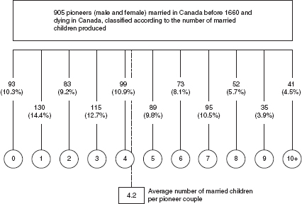
In 1608 Québec was founded and the French inhabitation of the St Lawrence Valley, virtually abandoned by the Iroquois, began. During the following century, approximately 15,000 immigrants arrived in these virgin lands from Normandy, from the area around Paris, and from central western France. Two-thirds of these returned to France after stays of varying lengths. The current population of 6 million French Canadians descends, for the most part, from those 5,000 immigrants who remained, as subsequent immigration contributed little to population growth. Thanks to a genealogic-demographic reconstruction carried out by a group of Canadian scholars, a considerable amount of information relating to demographic events is known about this population. For example, two pioneers, Jean Guyon and Mathurine Robin, had 2,150 descendants by 1730. Naturally, subsequent generations, including wives and husbands from other genealogical lines, contributed to this figure, which in and of itself has little demographic significance. On the other hand, the fate of another pioneer, the famous explorer Samuel de Champlain, was very different, and he left no descendants at all. The extraordinary Canadian material also provides measures of significant demographic interest. For example, the 905 pioneers (men and women) who were born in France, migrated to Canada before 1660, and both married and died in Canada, produced on average 4.2 married offspring per couple (), a level of fertility which corresponds to a doubling of the original population in a single generation (from two spouses, four married children). The exceptionally high reproductive capacity of the settlers of French Canada was the result of an extraordinary combination of circumstances: the physical selection of the immigrants, their high fertility and low mortality, ample available space, low density, and the absence of epidemics.
Growth of the French Canadian population (seventeenth century): pioneers and their children
We have unknowingly touched the heart of the mechanisms of population growth. As we have seen, a population grows (or declines or remains stationary) from one generation to the next if those who gain access to reproduction (here defined by the act of marriage) are in turn successful in bringing a larger (or smaller or equal) number of individuals to marriage. The end result, whatever it might be, is basically determined by two factors: the number of children each individual, or each couple, succeeds in producing – due to biological capability, desire, age at marriage, length of cohabitation, and other factors – and the intensity of mortality from birth until the end of the reproductive period. A familiarity with these mechanisms, which I shall discuss in the following section, is essential for understanding the factors of demographic change.
4 Reproduction and Survival
The growth potential of a population may be expressed as the function of two measures, whose significance should be intuitive: (1) the number of births, or children, per woman, and (2) life expectancy at birth. These are synthetic measures of, respectively, reproduction and survival. The first describes the average number of children produced by a generation of women during the course of their reproductive lives and in the hypothetical absence of mortality. Below we shall consider the biological, social, and cultural factors which determine the level of this measure. The second, life expectancy at birth, describes the average duration of life (or average number of years lived) for a generation of newborns and is a function of the force of mortality at the various ages, which in turn is determined by the species’ biological characteristics and relationship with the surrounding environment. In the primarily rural societies of past centuries, which lacked modern birth control and effective medical knowledge, both of these measures might vary considerably. The number of children per woman ranged from less than five to more than eight (though today, in some western societies characterized by high levels of birth control, it has declined below one), and life expectancy at birth ranged from 20 to 40 years (today it has exceeded 80 in some countries).
The number of children per woman depends, as has been said, on biological and social factors which determine: (1) the frequency of births during a woman’s fecund period, and (2) the portion of the fecund period – between puberty and menopause – effectively utilized for reproduction.
The frequency of births
This is an inverse function of the interval between births. Given the condition of natural fertility – a term used by demographers to describe those premodern societies which did not practice intentional contraception for the purpose of controlling either the number of births or their timing – the interval between births may be divided into four parts:
1 A period of infertility after every birth, as ovulation does not recommence for a couple of months. However, this anovulatory period, during which it is impossible to conceive, increases with the duration of breast-feeding, which is often continued until the second, and in some cases even third, year of the child’s life. The duration of breast-feeding, however, varies considerably from one culture to another, so much so that the minimum and maximum limits for the infertility period fall between 3 and 24 months.
2 The waiting time, which consists of the average number of months that pass between the resumption of normal ovulation and conception. It is possible that some women, either for accidental or natural reasons, may conceive during the first ovulatory cycle, while others, even given regular sexual relations, may not do so for many cycles. We can take five and ten months as our upper and lower limits.
3 The average length of pregnancy, which as everyone knows is about nine months.
4 Fetal mortality. About one out of every five recognized pregnancies does not come to term because of miscarriage. According to the few studies available, this seems to be a frequency which does not vary much from population to population. After a miscarriage, a new conception can take place after the normal waiting period (five to ten months). As only one in five conceptions contributes to this component of the birth interval, the average addition is one to two months.
Totaling the minimum and maximum values of 1, 2, 3, and 4, we find that the interval between births ranges from 18 to 45 months (or approximately 1.5 to 3.5 years), but, as a combination either of maxima or minima is improbable, this interval usually falls between two and three years. The above analysis holds true for a population characterized by uncontrolled, natural fertility. Of course, if birth control is introduced the reproductive life span without children may be expanded at will.
The fecund period used for reproduction
The factors that determine the age of access to reproduction, or the establishment of a stable union for the purpose of reproduction (marriage), are primarily cultural, while those that determine the age at which the reproductive period ends are primarily biological.
1 The age at marriage may vary between a minimum close to the age of puberty – let us say 15 years – and a maximum which in many European societies has exceeded 25.
2 The age at the end of the fecund period may be as high as 50, but on average is much lower. We can take as a good indicator the average age of mothers at the birth of the last child in populations that do not practice birth control. This figure is fairly stable and varies between 38 and 41.
We can say, then – again combining minima and maxima and rounding – that the average length of a union for reproductive purposes, barring death or divorce, may vary between 15 and 25 years.
Simplifying still more, we can estimate what the minimum and maximum levels of procreation might be in hypothetical populations not subject to mortality. To obtain the minimum we combine the minimum reproductive period (15 years) with the maximum birth interval (3.5 years).

To obtain the maximum level we instead combine the maximum reproductive period (25 years) with the minimum birth interval (1.5 years):

These combinations of extremes (especially the latter) are of course impossible, as the various components are not independent from one another. The repeated childbearing which follows early marriage, for example, can create pathological conditions which lower fecundity or else lead to an early decline in sexual activity and so increase the birth interval. In stable historical situations, average levels of under five or over eight children per woman are rare.
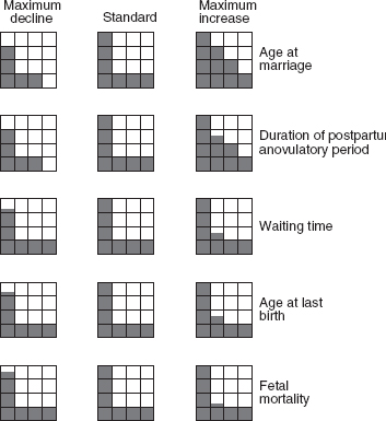
The number of children per woman depends primarily upon the age at marriage (the principal factor determining the length of the reproductive period) and the duration of breast-feeding (the principal component determining the birth interval). , borrowed from the Bongaarts and Menken article on which this discussion is based, shows how the average number of children per woman can vary as a result of the variation (between maximum and minimum values) of each component. We take as a standard seven children, obtained by combining average values of the various components. As one component varies the others remain fixed.
Effect on the average number of children per woman of maximum variations of the components of fertility above and below the standard (1 square = 1 birth)
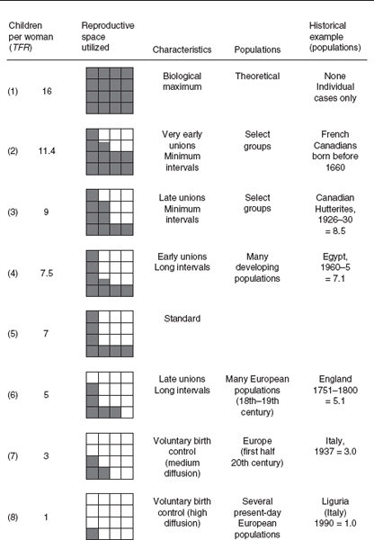
In the above model is applied to several historical (and theoretical) examples. In addition to the biological maximum (1), there are: a possible maximum (2) resulting from a combination of early marriage (at age 18) and short birth intervals (due to early weaning); a possible minimum in the absence of birth control (6) resulting from late marriage (at age 25) and prolonged breast-feeding; three intermediate levels (3), (4), and (5); and finally, examples of medium and very high levels of birth control, (7) and (8), yielding respectively three and one children. These examples should not be considered to represent a chronological or evolutionary sequence, as almost all can be found in populations living in the same historical periods (except for the last two, characterized by strongly controlled fertility, which can only be found in modern populations).
Fertility models
In addition to the biosocial components determining fertility, human reproductivity must also contend with the hard check of mortality, a factor that we have ignored up to this point. Reproductivity and mortality are not independent of one another for any living species, including humans. When the number of offspring is very large, the risk of death in early infancy increases and the competition for resources within the family can lower resistance at all ages. On the other hand, high fertility is in the long run incompatible with low, or recently lowered, mortality, given the resultant excessive population growth. Nonetheless, mortality is to a large degree rooted in human biology and so is independent of fertility levels.
A fairly simple way to describe human mortality is provided by the survivorship function, l x, which traces the progressive elimination of a generation of 10n individuals from birth to the age at which the last member dies. shows three survivorship curves. The lower curve corresponds to a life expectancy at birth (e 0) of 20 years. This is a very low figure, near to the minimum compatible with the continued survival of a population, and might characterize a primitive population living in a hostile environment. The upper curve corresponds to an e 0 of 83 years, a level that the more-developed countries are about to reach. The third, intermediate curve (e 0 = 50) is typical of those countries that have benefited from a limited degree of modern medical progress. In I have chosen as the maximum age, in all three cases, 100 years, assuming that this is the limit of human longevity. This assumption is not far from the truth, as considerably less than 1 percent of the initial generation survives to this age. Continuing to refer to , if we imagine that no one dies until their hundredth birthday, at which age everyone dies, then the l x curve will be rectangular (it will be parallel to the abscissa until age 100, at which point it will drop vertically to 0) and e 0 will be equal to 100. The life expectancies at birth described by the other curves are proportional to the areas under those curves. The shape of the survivorship curves depends upon the force of mortality at the various ages. In human populations there is a period of high mortality immediately after birth and during early infancy, the result of fragility in the face of the external environment. Mortality risk reaches a minimum during late infancy or adolescence and then, from maturity, rises exponentially as a function of the gradual weakening of the organism. In high-mortality regimes (see the e 0 = 20 curve) the curve tends to be concave up. As mortality improves, infant mortality becomes less of a factor and the curve becomes more and more concave down. From a strictly genetic point of view – the hereditary genetic transmission of characteristics – survival beyond the reproductive years (for simplicity, say 50 years of age) is of course irrelevant. However high or low it might be, the rate of mortality beyond age 50 will have no effect on the genetic patrimony of a population. Before and during the reproductive years, on the other hand, the higher the level of mortality, the stronger the selective effect, as individuals possessing characteristics unfavorable to survival are eliminated and so do not pass on these characteristics to subsequent generations.
Survival curves for three female populations characterized by low, medium, and high life expectancy at birth
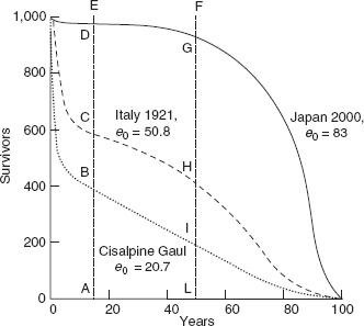
Note: Survival curves trace the numerical decline with age of a generation of 1,000 births. Life expectancy at birth is proportional to the space bounded by the ordinate, the abscissa, and the survival curve. The area AEFl, equal to 35 years, describes the length of the reproductive period. The areas ADGL, ACHL, and ABIL describe the average effective reproductive lives for the three generations of 1,000 newborn girls, equal to 34.4, 24.8, and 10.2 years. The ratios ADGL/AEFL, ACHL/AEFL, and ABIL/AEFL are, respectively, 98.2, 70.8, and 29.2 percent, and represent the average part of the reproductive period lived by the three generations.
Nonetheless, increased survival beyond the reproductive ages may have indirect biological effects, as older adults contribute to the accumulation, organization, and transmission of knowledge, while also favoring parental investments, and so can contribute to the improved survival of new generations.
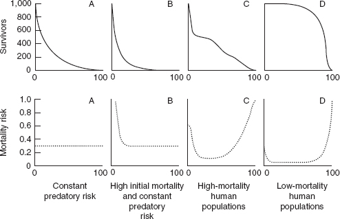
shows two survivorship models typical of other species, together with high- and low-mortality human models. Model A typifies those species that are subject to the relatively constant mortality risk presented by other predatory species, while model B is typical of those (r-strategy) species that depend upon prolific reproduction for survival and are subject to very high postnatal mortality.
Survival models
Let us return to the human species. In order to appreciate its reproductive capacity, we must understand the laws governing its survival until the end of the reproductive period. Afterward, whether or not an individual survives is theoretically unimportant. From we can see that, with life expectancy at birth equal to 20 years, only 29.2 percent of the potential fecund life of a generation is actually lived owing to the decimation caused by high mortality. This proportion increases gradually with increasing life expectancy (and the elevation of the l x curve). In the examples given, it is 70.8 percent when e 0 equals 50 and 98.2 percent when e 0 equals 80.
It should be clear now that the reproductive success of a population – and so its growth – depends upon the number of children born to those women who survive to reproductive age. If we imagine a level of six children per woman in the absence of mortality, then in that case where only 30 percent of the reproductive space is used (e 0 = 20) the number of children born per woman is 6 × 0.3 = 1.8. When e 0 = 50 and 70 percent of the reproductive space is used, the number of children is 6 × 0.7 = 4.2; and when 99 percent is used (e 0 = 83), the total is 6 × 0.99 = 5.94. Since there are two parents for every child, each hypothetical couple pays its demographic debt (and the number of parents and children is about equal) if our calculation above yields a level of two. A number larger than two implies growth. If the number of surviving children is four, then the population will double in the course of a single generation (about 30 years) and the average annual growth rate will be 2.3 percent.
5 The Space of Growth
Fertility and mortality, acting in tandem, impose objective limits on the pattern of growth of human populations. If we imagine that in a certain population these remain fixed for a long period of time, then, by resorting to a few simplifying hypotheses, we can express the rate of growth as a function of the number of children per woman (TFR) and life expectancy at birth (e 0).
shows several “isogrowth” curves. Each curve is the locus of those points that combine life expectancy (the abscissa) and number of children per woman (the ordinate) to give the same rate of growth r. Included on this graph are points corresponding to historical and contemporary populations. For the former, life expectancy is neither below 15, as this would be incompatible with the continued survival of the population, nor above 45, as no historical population ever achieved a higher figure. For similar reasons the number of children per woman falls between eight (almost never exceeded in normally constituted populations) and four (recall that these are populations not practicing birth control). reports, left to right, four areas, three ellipses and one round in shape; each of these areas represents the locus of populations belonging to different epochs. The first ellipse is the locus of historical populations before the Industrial Revolution and the modern diffusion of birth control. These populations fall within a band of growth rates that extends from 0 to 1 percent, a space of growth typical of pre-modern times. Within this narrow band, however, the fertility and mortality combinations vary widely, although constrained by the syndromic poverty of resources and of knowledge. Denmark at the end of the eighteenth century and India a century later, for example, have similar growth rates, but these are achieved at distant points in the strategic space described: the former example combines high life expectancy (about 40 years) and a small number of children (just over four), while in the latter case low life expectancy (about 25 years) is paired with many children (just under seven).
Relationship between the average number of children per woman (TFR) and life expectancy (e 0) in historical and present-day populations
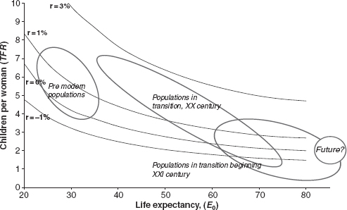
Although their growth rates must have been similar, the points for Paleolithic and Neolithic populations are assumed to have been far apart. According to a well-accepted opinion (see Chapter 2), the Paleolithic, a hunting and gathering population, was characterized by lower mortality, owing to its low density, a factor that prevented infectious diseases from taking hold and spreading, and moderate fertility, compatible with its nomadic behavior. For the Neolithic, a sedentary and agricultural population, both mortality and fertility were higher as a result of higher density and lower mobility.
The second ellipse contains the populations during the process of demographic transition in the twentieth century. The strategic space utilized, previously restricted to a narrow band, has expanded dramatically. Medical and sanitary progress has shifted the upper limit of life expectancy from the historical level of about 40 years to the present level above 80, while the introduction of birth control has reduced the lower limit of fertility to a level of about one child per woman. The third ellipse outlines the situation at the beginning of the twenty-first century, when countries with very high fertility (many in sub-Saharan Africa) coexist with other countries (in Europe and Southern and Eastern Asia) with abnormally low fertility, close to one child per woman. It must be remarked that in the much expanded space of the twentieth and twenty-first centuries there are populations with implicit growth rates of 4 percent, and other populations with negative growth rates of −2 percent. A population with a 4 percent rate of growth doubles in 17–18 years, and one declining at the rate of 2 percent halves in 35 years. Two populations of equal size experiencing these different growth rates will find themselves after 35 years (about a generation) in a numerical ratio of eight-to-one! However, this is the space of populations in transition, unstable, and often with unsustainable paces of growth. The fourth space, circular in shape, is the hypothetical region of the future, after the transition and at the end of a process of convergence, with an expectation of life above 80, fertility between 1 and 3 children per woman, and potential rates of growth between −1 and + 1 percent. These populations could alternate phases of growth and decline, possibly not synchronized, with relatively small and diluted changes in time.
6 Environmental Constraints