Cover

John Wiley & Sons Ltd, The Atrium, Southern Gate, Chichester, West Sussex, PO19 8SQ, United Kingdom

For details of our global editorial offices, for customer services and for information about how to apply for permission to reuse the copyright material in this book please see our website at www.wiley.com.

The right of the author to be identified as the author of this work has been asserted in accordance with the Copyright, Designs and Patents Act 1988.

All rights reserved. No part of this publication may be reproduced, stored in a retrieval system, or transmitted, in any form or by any means, electronic, mechanical, photocopying, recording or otherwise, except as permitted by the UK Copyright, Designs and Patents Act 1988, without the prior permission of the publisher.

Wiley also publishes its books in a variety of electronic formats. Some content that appears in print may not be available in electronic books.

Designations used by companies to distinguish their products are often claimed as trademarks. All brand names and product names used in this book are trade names, service marks, trademarks or registered trademarks of their respective owners. The publisher is not associated with any product or vendor mentioned in this book. This publication is designed to provide accurate and authoritative information in regard to the subject matter covered. It is sold on the understanding that the publisher is not engaged in rendering professional services. If professional advice or other expert assistance is required, the services of a competent professional should be sought.

Preface

Mathematical programmes are among the most widely used models in operational research and management science. In many cases their application has been so successful that their use has passed out of operational research departments to become an accepted routine planning tool. It is therefore rather surprising that comparatively little attention has been paid in the literature to the problems of formulating and building mathematical programming models or even deciding when such a model is applicable. Most published work has tended to be of two kinds. Firstly, case studies of particular applications have been described in the operational research journals and journals relating to specific industries. Secondly, research work on new algorithms for special classes of problems has provided much material for the more theoretical journals. This book attempts to fill the gap by, in Part I, discussing the general principles of model building in mathematical programming. In Part II, 29 practical problems are presented to which mathematical programming can be applied. By simplifying the problems, much of the tedious institutional detail of case studies is avoided. It is hoped, however, that the essence of the problems is preserved and easily understood. Finally, in Parts III and IV, suggested formulations and solutions to the problems are given together with some computational experience.

Many books already exist on mathematical programming or, in particular, linear programming. Most such books adopt the conventional approach of paying a great deal of attention to algorithms. Since the algorithmic side has been so well and fully covered by other texts, it is given much less attention in this book. The concentration here is more on the building and interpreting of models rather than on the solution process. Nevertheless, it is hoped that this book may spur the reader to delve more deeply into the often challenging algorithmic side of the subject as well. It is, however, the author's contention that the practical problems and model building aspect should come first. This may then provide a motivation for finding out how to solve such models. Although desirable, knowledge of algorithms is no longer necessary if practical use is to be made of mathematical programming. The solution of practical models is now largely automated by the use of commercial package programs that are discussed in Chapter 2.

For the reader with some prior knowledge of mathematical programming, parts of this book may seem trivial and can be skipped or read quickly. Other parts are, however, rather more advanced and present fairly new material. This is particularly true of the chapters on integer programming. Indeed, this book can be treated in a nonsequential manner. There is much cross-referencing to enable the reader to pass from one relevant section to another. This book is aimed at three types of readers:

1. It is intended to provide students in universities and polytechnics with a solid foundation in the principles of model building as well as the more mathematical, algorithmic side of the subject, which is conventionally taught. For students who finally go on to use mathematical programming to solve real problems, the model building aspect is probably the more important. The problems in Part II provide practical exercises in problem formulation. By formulating models and solving them with the aid of a computer, students learn the art of formulation in the most satisfying way possible. They can compare their numerical solutions with those of other students obtained from differently build models. In this way they learn how to validate a model.

It is also hoped that these problems will be of use to research students seeking new algorithms for solving mathematical programming problems. Very often they have to rely on trivial or randomly generated models to test their computational procedures. Such models are far from typical of those found in the real world. Moreover, they are one (or more) steps removed from practical situations. They therefore obscure the need for efficient formulations as well as algorithms.

2. This book is also intended to provide managers with a fairly nontechnical appreciation of the scope and limitations of mathematical programming. In addition, by looking at the practical problems described in Part II they may recognize a situation in their own organization to which they had not realized mathematical programming could be applied.

3. Finally, constructing a mathematical model of an organization provides one of the best methods of understanding that organization. It is hoped that the general reader will be able to use the principles described in this book to build mathematical models and thereby learn about the functioning of systems, which purely verbal descriptions fail to explain. It has been the author's experience that the process of building a model of an organization can often be more beneficial even than the obtaining of a solution. A greater understanding of the complex interconnections between different facets of an organization is forced upon anybody who realistically attempts to model that organization.

Part I of this book describes the principles of building mathematical programming models and how they may arise in practice. In particular, linear programming, integer programming and separable programming models are described. A discussion of the practical aspects of solving such models and a very full discussion of the interpretation of their solutions is included.

Part II presents each of the 29 practical problems in sufficient detail to enable the reader to build a mathematical programming model using the numerical data. In some cases the origin of the problem is mentioned.

Part III discusses each problem in detail and presents a possible formulation as a mathematical programming model.

Part IV gives the optimal solutions obtained from the formulations presented in Part III. Some computational experience is also given in order to give the reader some feel of the computational difficulty of solving the particular type of model.

It is hoped that readers will attempt to formulate and possibly solve the problems for themselves before proceeding to Parts III and IV.

By presenting 29 problems from widely different contexts the power of the technique of mathematical programming in giving a method of tackling them all should be apparent. Some problems are intentionally “unusual” in the hope that they may suggest the application of mathematical programming in rather novel areas.

Many references are given at the end of the book. The list is not intended to provide a complete bibliography of the vast number of case studies published. Many excellent case studies have been ignored. The list should, however, provide a representative sample which can be used as a starting point for a deeper search into the literature.

Many people have both knowingly and unknowingly helped in the preparation of successive editions of this book with their suggestions and opinions. In particular I would like to thank Gautam Appa, Sheena and Robert Ashford, Martin Beale, Tony Brearley, Ian Buchanan, Colin Clayman, Lewis Corner, Martyn Jeffreys, Bob Jeroslow, Clifford Jones, Bernard Kemp, Ailsa Land, Adolfo Fonseca Manjarres, Kenneth McKinnon, Gautam Mitra, Heiner Müller-Merbach, Bjorn Nygreen, Pat Rivett, Richard Thomas, Steven Vajda and Will Watkins. I must express a great debt of gratitude to Robin Day of Edinburgh University, whose deep computing knowledge and programming ability helped me immensely in building the models for early editions of this book and implementing our design of the modelling system MAGIC. This has now been replaced by the system NEWMAGIC, which has been written by George Skondras. It is available with the optimizer EMSOL. All the models in the book have been built and solved in this system. The models, formulated in Part III, have been modelled in the NEWMAGIC language and are available on the website: www.wiley.com/go/model_building_mathematical_programming

Since the first edition was written, computational power has increased immensely. Solution times for the models are therefore, in most cases, of little relevance and are ignored. A few of the models are still difficult to solve. In these cases, some computational experience is given.

The fourth edition has been enhanced by new sections or models on Constraint Logic Programming, Data Envelopment Analysis, Hydro Electricity Generation, Milk Distribution and Yield Management in an airline together with state-of-the-art material and extra references on a number of topics and applications. I am very grateful to Kenneth McKinnon for advice and help with these models.

It is gratifying to know how well this book has been received together with the demand for a fourth edition.

Preface to the Fifth Edition

The fifth edition includes new sections on Stochastic Programming and Column Generation, a subsection on the Vehicle Routing problem and an enhanced section on Constraint Logic Programming. In addition, the subsection on modelling nonlinear functions and constraints, by integer variables, has been improved with a more versatile formulation. Many other small clarifications and improvements have also been included.

Five new problems have been added: a Car Rental and Return problem and an extension, an Airport Lost Baggage Distribution problem and two problems in Molecular Biology.

New references have been added, although it is recognized that it is impossible to mention all the excellent papers that have been written since earlier editions of this book. I apologize to the many authors of these papers who have not been cited.

A number of people have given me advice on improving and correcting the fourth edition to produce this fifth edition. In particular, I would like to mention Harvey Greenberg, John Hooker, Cormac Lucas, Andrew McGee and Ken McKinnon. They have all helped validate the new material. Also, a number of correspondents have pointed out small typos. I am grateful to them all.

Chapter 1

Introduction

1.1 The concept of a model

Many applications of science make use of models. The term ‘model’ is usually used for a structure that has been built with the purpose of exhibiting features and characteristics of some other objects. Generally, only some of these features and characteristics will be retained in the model depending upon the use to which it is to be put. Sometimes, such models are concrete, as is a model aircraft used for wind tunnel experiments. More often, in operational research, we will be concerned with abstract models. These models will usually be mathematical in that algebraic symbolism will be used to mirror the internal relationships in the object (often an organization) being modelled. Our attention will mainly be confined to such mathematical models, although the term ‘model’ is sometimes used more widely to include purely descriptive models.

The essential feature of a mathematical model in operational research is that it involves a set of mathematical relationships (such as equations, inequalities and logical dependencies) that correspond to some more down-to-earth relationships in the real world (such as technological relationships, physical laws and marketing constraints).

1. The actual exercise of building a model often reveals relationships that were not apparent to many people. As a result, a greater understanding is achieved of the object being modelled.

2. Having built a model it is usually possible to analyse it mathematically to help suggest courses of action that might not otherwise be apparent.

3. Experimentation is possible with a model, whereas it is often not possible or desirable to experiment with the object being modelled. It would clearly be politically difficult, as well as undesirable, to experiment with unconventional economic measures in a country if there were a high probability of disastrous failure. The pursuit of such courageous experiments would be more (though not perhaps totally) acceptable on a mathematical model.

It is important to realize that a model is really defined by the relationships that it incorporates. These relationships are, to a large extent, independent of the data in the model. A model may be used on many different occasions with differing data, for example, costs, technological coefficients and resource availabilities. We would usually still think of it as the same model even though some coefficients have been changed. This distinction is not, of course, total. Radical changes in the data would usually be thought of as a change in the relationships and therefore the model.

Many models used in operational research (and other areas such as engineering and economics) take standard forms. The mathematical programming type of model that we consider in this book is probably the most commonly used standard type of model. Other examples of some commonly used mathematical models are simulation models, network planning models, econometric models and time series models. There are many other types of model, all of which arise sufficiently often in practice to make them areas worthy of study in their own right. It should be emphasized, however, that any such list of standard types of model is unlikely to be exhaustive or exclusive. There are always practical situations that cannot be modelled in a standard way. The building, analysing and experimenting with such new types of model may still be a valuable activity. Often, practical problems can be modelled in more than one standard way (as well as in non-standard ways). It has long been realized by operational research workers that the comparison and contrasting of results from different types of model can be extremely valuable.

Many misconceptions exist about the value of mathematical models, particularly when used for planning purposes. At one extreme, there are people who deny that models have any value at all when put to such purposes. Their criticisms are often based on the impossibility of satisfactorily quantifying much of the required data, for example, attaching a cost or utility to a social value. A less severe criticism surrounds the lack of precision of much of the data that may go into a mathematical model; for example, if there is doubt surrounding 100 000 of the coefficients in a model, how can we have any confidence in an answer it produces? The first of these criticisms is a difficult one to counter and has been tackled at much greater length by many defenders of cost–benefit analysis. It seems undeniable, however, that many decisions concerning unquantifiable concepts, however, they are made, involve an implicit quantification that cannot be avoided. Making such a quantification explicit by incorporating it in a mathematical model seems more honest as well as scientific. The second criticism concerning accuracy of the data should be considered in relation to each specific model. Although many coefficients in a model may be inaccurate, it is still possible that the structure of the model results in little inaccuracy in the solution. This subject is mentioned in depth in Sections 4.2 and 6.3.

At the opposite extreme to the people who utter the above criticisms are those who place an almost metaphysical faith in a mathematical model for decision-making (particularly if it involves using a computer). The quality of the answers that a model produces obviously depends on the accuracy of the structure and data of the model. For mathematical programming models, the definition of the objective clearly affects the answer as well. Uncritical faith in a model is obviously unwarranted and dangerous. Such an attitude results from a total misconception of how a model should be used. To accept the first answer produced by a mathematical model without further analysis and questioning should be very rare. A model should be used as one of a number of tools for decision-making. The answer that a model produces should be subjected to close scrutiny. If it represents an unacceptable operating plan, then the reasons for unacceptability should be spelled out and if possible incorporated in a modified model. Should the answer be acceptable, it might be wise only to regard it as an option. The specification of another objective function (in the case of a mathematical programming model) might result in a different option. By successive questioning of the answers and altering the model (or its objective), it should be possible to clarify the options available and obtain a greater understanding of what is possible.

1.2 Mathematical programming models

It should be pointed out immediately that mathematical programming is very different from computer programming. Mathematical programming is ‘programming’ in the sense of ‘planning’. As such, it need have nothing to do with computers. The confusion over the use of the word ‘programming’ is widespread and unfortunate. Inevitably, mathematical programming becomes involved with computing as practical problems almost always involve large quantities of data and arithmetic that can only reasonably be tackled by the calculating power of a computer. The correct relationship between computers and mathematical programming should, however, be understood.

The common feature that mathematical programming models have is that they all involve optimization. We wish to maximize something or minimize something. The quantity that we wish to maximize or minimize is known as an objective function. Unfortunately, the realization that mathematical programming is concerned with optimizing an objective often leads people summarily to dismiss mathematical programming as being inapplicable in practical situations where there is no clear objective or there are a multiplicity of objectives. Such an attitude is often unwarranted because, as we shall see in Chapter 3, there is often value in optimizing some aspect of a model when in real life there is no clear-cut single objective.

In this book, we confine our attention to some special types of mathematical programming model. These can most easily be classified as linear programming (LP) models, non-linear programming (NLP) models and integer programming (IP) models. We begin by describing what an LP model is by means of two small examples.

Example 1.1: A Linear Programming (LP) Model (Product Mix)

An engineering factory can produce five types of product (PROD 1, PROD 2, …, PROD 5) by using two production processes: grinding and drilling.

After deducting raw material costs, each unit of each product yields the following contributions to profit:

Each unit requires a certain time on each process. These are given below (in hours). A dash indicates when a process is not needed.

In addition, the final assembly of each unit of each product uses 20 hours of an employee's time.

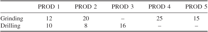
The factory has three grinding machines and two drilling machines and works a six-day week with two shifts of 8 hours on each day. Eight workers are employed in assembly, each working one shift a day.

The problem is to find how much of each product is to be manufactured so as to maximize the total profit contribution.

This is a very simple example of the so-called ‘product mix’ application of LP.

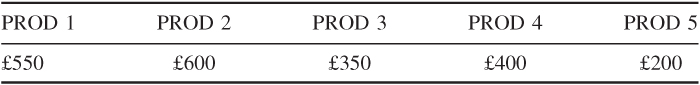
In order to create a mathematical model, we introduce variables x₁, x₂, …, x₅ representing the numbers of PROD 1, PROD 2, …, PROD 5 that should be produced in a week. As each unit of PROD 1 yields £550 contribution to profit and each unit of PROD 2 yields £600 contribution to profit, etc., our total profit contribution will be represented by the expression:

The objective of the factory is to choose x₁, x₂, …, x₅ so as to make the value of this expression as high as possible, that is, Expression (1.1) is the objective function that we wish to maximize (in this case).

Clearly, our processing and labour capacities, to some extent, limit the values that the x_j can take. Given that we have only three grinding machines working for a total of 96 hours a week each, we have 288 hours of grinding capacity available. Each unit of PROD 1 uses 12 hours grinding. x₁ units will therefore use 12x₁ hours. Similarly, x₂ units of PROD 2 will use 20x₂ hours. The total amount of grinding capacity that we use in a week is given by the expression on the left-hand side of Inequality (1.2):

Inequality (1.2) is a mathematical way of saying that we cannot use up more than the 288 hours of grinding available per week. Inequality (1.2) is known as a constraint. It restricts (or constrains) the possible values that the variables x_j can take.

The drilling capacity is 192 hours a week. This gives rise to the following constraint:

Finally, the fact that we have only a total of eight assembly workers each working 48 hours a week gives us a labour capacity of 384 hours. As each unit of each product uses 20 hours of this capacity, we have the constraint

We have now expressed our original practical problem as a mathematical model. The particular form that this model takes is that of an LP model. This model is now a well-defined mathematical problem. We wish to find values for the variables x₁, x₂, …, x₅ that make expression (1.1) (the objective function) as large as possible but still satisfy constraints (1.2)–(1.4). You should be aware of why the term ‘linear’ is applied to this particular type of problem. Expression (1.1) and the left-hand sides of constraints (1.2)–(1.4) are all linear. Nowhere do we get terms like

, x₁x₂ or log x appearing.

There are a number of implicit assumptions in this model that we should be aware of. Firstly, we must obviously assume that the variables x₁, x₂, …, x₅ are not allowed to be negative, that is, we do not make negative quantities of any product. We might explicitly state these conditions by the extra constraints

In most LP models the non-negativity constraints (1.5) are implicitly assumed to apply unless we state otherwise. Secondly, we have assumed that the variables x₁, x₂, …, x₅ can take fractional values, for example, it is meaningful to make 2.36 units of PROD 1. This assumption may or may not be entirely warranted. If, for example, PROD 1 represented gallons of beer, fractional quantities would be acceptable. On the other hand, if it represented numbers of motor cars, it would not be meaningful. In practice, the assumption that the variables can be fractional is perfectly acceptable in this type of model, if the errors involved in rounding to the nearest integer are not great. If this is not the case, we have to resort to IP.

1. There is a single linear expression (the objective function) to be maximized or minimized.

2. There is a series of constraints in the form of linear expressions, which must not exceed (≤) some specified value. LP constraints can also be of the form ‘≥’ and ‘=’, indicating that the value of certain linear expressions must not fall below a specified value or must exactly equal a specified value.

3. The set of coefficients 288, 192, 384, on the right-hand sides of constraints (1.2)–(1.4), is generally known as the right-hand side column.

Practical models will, of course, be much bigger (more variables and constraints) and more complicated but they must always have the above three essential features. The optimal solution to the above model is included in Section 6.2.

In order to give a wider picture of how LP models can arise, we give a second small example of a practical problem.

Example 1.2: A Linear Programming Model (Blending)

A food is manufactured by refining raw oils and blending them together. The raw oils come in two categories:

Vegetable oils	VEG 1 VEG 2
Non-vegetable oils	OIL 1 OIL 2 OIL 3

Vegetable oils and non-vegetable oils require different production lines for refining. In any month, it is not possible to refine more than 200 tons of vegetable oil and more than 250 tons of non-vegetable oils. There is no loss of weight in the refining process and the cost of refining may be ignored.

There is a technological restriction of hardness in the final product. In the units in which hardness is measured, this must lie between 3 and 6. It is assumed that hardness blends linearly. The costs (per ton) and hardness of the raw oils are

The final product sells for £150 per ton.

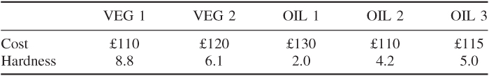
How should the food manufacturer make their product in order to maximize their net profit?

This is another very common type of application of LP although, of course, practical problems will be, generally, much bigger.

Variables are introduced to represent the unknown quantities. x₁, x₂, …, x₅ represent the quantities (tons) of VEG 1, VEG 2, OIL 1, OIL 2 and OIL 3 that should be bought, refined and blended in a month. y represents the quantity of the product that should be made. Our objective is to maximize the net profit:

The hardness limitations on the final product are imposed by the following two constraints:

Finally it is necessary to make sure that the weight of the final product is equal to the weight of the ingredients. This is done by a continuity constraint:

The objective function (1.6) (to be maximized) together with constraints (1.7–(1.11) make up our LP model.

The linearity assumption of LP is not always warranted in a practical problem, although it makes any model computationally much easier to solve. When we have to incorporate non-linear terms in a model (either in the objective function or the constraints) we obtain an non-linear programming (NLP) model. In Chapter 7, we will see how such models may arise and a method of modelling a wide class of such problems using separable programming. Nevertheless, such models are usually far more difficult to solve.

Finally, the assumption that variables can be allowed to take fractional values is not always warranted. When we insist that some or all of the variables in an LP model must take integer (whole number) values we obtain an integer programming (IP) model. Such models are again much more difficult to solve than conventional LP models. We will see in Chapters 8–10 that IP opens up the possibility of modelling a surprisingly wide range of practical problems.

Another type of model that we discuss in Section 4.2 is known as a stochastic programming model. This arises when some of the data are uncertain but can be specified by a probability distribution. Although data in many LP models may be uncertain, their representation by expected values alone may not be sufficient. Situations in which a more explicit recognition of the probabilistic nature of data may be made, but the resultant model still converted to a linear program, are described. In Chapter 3, we mention chance-constrained models and in Chapter 4, multi-staged models with recourse, both of which fall in the category of stochastic programming. An example of the use of this latter type of model is given in Sections 12.24, 13.24 and 14.24 where it is applied to determining the price of airline tickets over successive periods in the face of uncertain demand. A good reference to stochastic programming is Kall and Wallace (1994).

Chapter 2

Solving mathematical programming models

2.1 Algorithms and packages

A set of mathematical rules for solving a particular class of problem or model is known as an algorithm. We are interested in algorithms for solving linear programming (LP), separable programming and integer programming IP models. An algorithm can be programmed into a set of computer routines for solving the corresponding type of model assuming the model is presented to the computer in a specified format. For algorithms that are used frequently, it turns out to be worth writing very sophisticated and efficient computer programmes for use with many different models. Such programmes usually consist of a number of algorithms collected together as a ‘package’ of computer routines. Many such package programmes are available commercially for solving mathematical programming models. They usually contain algorithms for solving LP models, separable programming models and IP models. These packages are written by computer manufacturers, consultancy firms and software houses. They are frequently very sophisticated and represent many person-years of programming effort. When a mathematical programming model is built, it is usually worth making use of an existing package to solve it rather than getting diverted onto the task of programming the computer to solve the model oneself.

The algorithms that are almost invariably used in commercially available packages are (i) the revised simplex algorithm for LP models; (ii) the separable extension of the revised simplex algorithm for separable programming models; and (iii) the branch and bound algorithm for IP models.

It is beyond the scope of this book to describe these algorithms in detail. Algorithms (i) and (ii) are well described in Beale (1968). Algorithm (iii) is outlined in Section 8.3 and well described in Nemhauser and Wolsey (1988). Although the above three algorithms are not the only methods of solving the corresponding models, they have proved to be the most efficient general methods. It should also be emphasized that the algorithms are not totally independent. Hence, the desirability of incorporating them in the same package. Algorithm (ii) is simply a modification of (i) and would use the same computer programme that would make the necessary changes in execution on recognizing a separable model. Algorithm (iii) uses (i) as its first phase and then performs a tree search procedure as described in Section 8.3.

One of the advantages of package programmes is that they are generally very flexible to use. They contain many procedures and options that may be used or ignored as the user thinks fit. We outline some of the extra facilities which most packages offer besides the three basic algorithms mentioned above.

2.1.1 Reduction

Some packages have a procedure for detecting and removing redundancies in a model and so reducing its size and hence time to solve. Such procedures usually go under the name REDUCE, PRESOLVE or ANALYSE. This topic is discussed further in Section 3.4.

2.1.2 Starting solutions

Most packages enable a user to specify a starting solution for a model if he/she wishes. If this starting solution is reasonably close to the optimal solution, the time to solve the model can be reduced considerably.

2.1.3 Simple bounding constraints

A particularly simple type of constraint that often occurs in a model is of the form

where U is a constant. For example, if x represented a quantity of a product to be made, U might represent a marketing limitation. Instead of expressing such a constraint as a conventional constraint row in a model, it is more efficient simply to regard the variable x as having an upper bound of U. The revised simplex algorithm has been modified to cope with such a bound algorithmically (the bounded variable version of the revised simplex). Lower bound constraints such as

need not be specified as conventional constraint rows either but may be dealt with analogously. Most computer packages can deal with bounds on variables in this way.

2.1.4 Ranged constraints

It is sometimes necessary to place upper and lower bounds on the level of some activity represented by a linear expression. This could be done by two constraints such as

A more compact and convenient way to do this is to specify only the first constraint above together with a range of b₁–b₂ on the constraint. The effect of a range is to limit the slack variable (which will be introduced into the constraint by the package) to have an upper bound of b₁–b₂, so implying the second of the above constraints. Most commercial packages have the facility for defining such ranges (not to be confused with ranging in sensitivity analysis, discussed below) on constraints.

2.1.5 Generalized upper bounding constraints

are very common in many LP models. Such a constraint is sometimes referred to by saying that there is a generalized upper bound (GUB) of M on the set of variables (x₁, x₂, …, x_n). If a considerable proportion of the constraints in a model are of this form and each such set of variables is exclusive of variables in any other set, then it is efficient to use the so-called GUB extension of the revised simplex algorithm. When this is used, it is not necessary to specify these constraints as rows of the model but treat them in a slightly analogous way to simple bounds on single variables. The use of this extension to the algorithm usually makes the solution of a model far quicker.

2.1.6 Sensitivity analysis

When the optimal solution of a model is obtained, there is often interest in investigating the effects of changes in the objective and right-hand side coefficients (and sometimes other coefficients) on this solution. Ranging is the name of a method of finding limits (ranges) within which one of these coefficients can be changed to have a predicted effect on the solution. Such information is very valuable in performing a sensitivity analysis on a model. This topic is discussed at length in Section 6.3 for LP models. Almost all commercial packages have a range facility.

2.2 Practical considerations

In order to demonstrate how a model is presented to a computer package and the form in which the solution is presented, we will consider the second example given in Section 1.2. This blending problem is obviously much smaller than most realistic models but serves to show the form in which a model might be presented.

This problem was converted into a model involving five constraints and six variables. It is convenient to name the variables VEG 1, VEG 2, OIL 1, OIL 2, OIL 3 and PROD. The objective is conveniently named PROF (profit) and the constraints VVEG (vegetable refining), NVEG (non-vegetable refining), UHAR (upper hardness), LHAR (lower hardness) and CONT (continuity). The data are conveniently drawn up in the matrix presented in Table 2.1. It will be seen that the right-hand side coefficients are regarded as a column and named CAP (capacity). Blank cells indicate a zero coefficient.

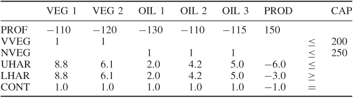
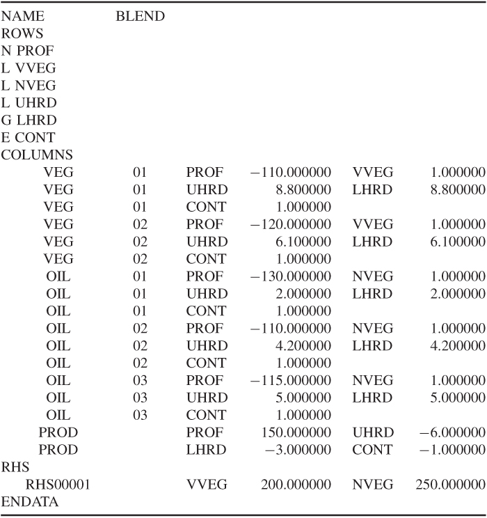
The information in Table 2.1 would generally be presented to the computer through a modelling language. There is, however, a standard format for presenting such information to most computer packages, and almost all modelling languages could convert a model to this format. This is known as MPS (mathematical programming system) format. Other format designs exist, but MPS format is the most universal. The presented data would be as in Table 2.1.

These data are divided into three main sections: the ROWS section, the COLUMNS section and the RHS section. After naming the problem BLEND, the ROWS section consists of a listing of the rows in the model together with a designator N, L, G or E. N stands for a non-constraint row—clearly the objective row must not be a constraint; L stands for a less-than-or-equal (≤) constraint; G stands for a greater-than-or-equal (≥) constraint; E stands for an equality (=) constraint. The COLUMNS section contains the body of the matrix coefficients. These are scanned column by column with up to two non-zero coefficients in a statement (zero coefficients are ignored). Each statement contains the column name, row names and corresponding matrix coefficients. Finally, the RHS section is regarded as a column using the same format as the COLUMNS section. The ENDATA entry indicates the end of the data.

Clearly, it may sometimes be necessary to put in other data as well (such as bounds). The format for such data can always be found from the appropriate manual for a package.

With large models, the solution procedures used will probably be more complicated than the standard ‘default’ methods of the package being used. There are many refinements to the basic algorithms which the user can exploit if he or she thinks it desirable. It should be emphasized that there are few hard-and-fast rules concerning when these modifications should be used. A mathematical programming package should not be regarded as a ‘black box’ to be used in the same way with every model on all computers. Experience with solving the same model again and again on a particular computer with small modifications to the data should enable the user to understand what algorithmic refinements prove efficient or inefficient with the model and computer installation. Experimentation with different strategies and even different packages is always desirable if a model is to be used frequently.

One computational consideration that is very important with large models is mentioned briefly. This concerns starting the solution procedure at an intermediate stage. There are two main reasons why one might wish to do this. First, one might be resolving a model with slightly modified data. Clearly, it would be desirable to exploit one's knowledge of a previous optimal solution to save computation in obtaining the new optimal solution. With linear and separable programming models, it is usually fairly easy to do this with a package, although it is much more difficult for IP models. Most packages have the facility to SAVE a solution on a file. Through the control programme, it is usually possible to RESTORE (or REINSTATE) such a solution as the starting point for a new run. A second reason for wishing to SAVE and RESTORE solutions is that one may wish to terminate a run prematurely. Possibly, the run may be taking a long time and a more urgent job has to go on the computer. Alternatively, the calculations may be running into numerical difficulty and have to be abandoned. In order not to waste the (sometimes considerable) computer time already expended, the intermediate (non-optimal) solution obtained just before termination can be saved and used as a starting point for a subsequent run. It is common to save intermediate solutions at regular intervals in the course of a run. In this way, the last such solution before termination is always available.

2.3 Decision support and expert systems

Some mathematical programming algorithms are incorporated in computer software designed for specific applications. Such systems are sometimes referred to as decision support systems. Often, they are incorporated into management information systems. They usually perform a large number of other functions as well as, possibly, solving a model. These functions probably include accessing databases and interacting with managers or decision makers in a ‘user friendly’ manner. If such systems do incorporate mathematical programming algorithms then many of the modelling and algorithmic aspects are removed from the user who can concentrate on their specific application. In designing and writing such systems, however, it is obviously necessary to automate many of the model building and interpreting procedures discussed in this book.

As decision support systems become more sophisticated, they are likely to present users with possible choices of decision besides the simpler tasks of storing, structuring and presenting data. Such choices may well necessitate the use of mathematical programming, although this function will be hidden from the user.

Another related concept in computer applications software is that of expert systems. These systems also pay great attention to the user interface. They are, for example, sometimes designed to accept ‘informal problem definitions’ and by interacting with users, to help them build up a more precise definition of the problem, possibly in the form of a model. This information is combined with ‘expert’ information built up in the past in order to help decision making. The computational procedures used often involve mathematical programming concepts (e.g. tree searches in IP as described in Section 8.3). While expert systems are beyond the scope of this book, the design and writing of such systems should again depend on mathematical programming and modelling concepts.

The use of mathematical programming in artificial intelligence and expert systems, in particular, is described by Jeroslow (1985) and Williams (1987).

2.4 Constraint programming (CP)

This is a different approach to solving many problems that can also be solved by IP. It is also, sometimes, known as constraint satisfaction or finite domain programming. While the methods used can be regarded as less sophisticated, in a conventional mathematical sense, they use more sophisticated computer science techniques. They have representational advantages that can make problems easier to model and, sometimes, easier to solve in view of the more concise representation. Therefore, we discuss the subject here. It seems likely that hybrid systems will eventually emerge in which the modelling capabilities of constraint programming (CP) are used in modelling languages for systems that use either CP or IP for solving the models. The integration of the two approaches is discussed by Hooker (2011) who has helped to design such a system SIMPL (Yunes et al. (2010)).

In CP, each variable has a finite domain of possible values. Constraints connect (or restrict) the possible combinations of values that the variables can take. These constraints are of a richer variety than the linear constraints of IP (although these are also included) and are usually expressed in the form of predicates, which must be true or false. They are also known as global (or meta) constraints since they are applied (if used) to the model as a whole and incorporated in the CP system used. That is in contrast to ‘local’ or ‘procedural’ constraints which can be constructed by the user to aid the solution process. Conventional IP models use only declarative constraints, so making a clear distinction between the statement of the model and the solution procedure. For illustration, we give some of the more common global constraints that are used in CP systems (often with different names).

all_different (x₁, x₂, …, x_n) means that all the variables in the predicate must take distinct values. While this condition can be modelled by a conventional IP formulation, it is more cumbersome. Once one of the variables has been set to one of the values in its domain (either temporarily or permanently), this predicate implies that the value must be taken out of the domain of the other variables (a process known as constraint propagationdomain reductionbound reduction