STATISTICAL ANALYSIS WITH MISSING DATA

2.6. Least Squares Estimates of Missing Values by ANCOVA Using Only Complete-Data Methods

2.7. Correct Least Squares Estimates of Standard Errors and One Degree of Freedom Sums of Squares

5.2. Imputation Methods that Provide Valid Standard Errors from a Single Filled-in Data Set

6.3. A Generally Flawed Alternative to Maximum Likelihood: Maximizing Over the Parameters and the Missing Data

7.2. Bivariate Normal Data with One Variable Subject to Nonresponse: ML Estimation

8. Maximum Likelihood for General Patterns of Missing Data: Introduction and Theory with Ignorable Nonresponse

9.2. Standard Errors via Methods that do not Require Computing and Inverting an Estimate of the Observed Information Matrix

PART III LIKELIHOOD-BASED APPROACHES TO THE ANALYSIS OF INCOMPLETE DATA: SOME EXAMPLES

11.2. Inference for a Mean Vector and Covariance Matrix with Missing Data Under Normality

13. Models for Partially Classified Contingency Tables, Ignoring the Missing-Data Mechanism

13.3. ML and Bayes Estimation for Multinomial Samples with General Patterns of Missing Data

14. Mixed Normal and Non-normal Data with Missing Values, Ignoring the Missing-Data Mechanism

14.4. Regression Problems Involving Mixtures of Continuous and Categorical Variables

15.3. Models with Known Nonignorable Missing-Data Mechanisms: Grouped and Rounded Data

Editors: David J. Balding, Peter Bloomfield, Noel A. C. Cressie, Nicholas I. Fisher, Iain M. Johnstone, J. B. Kadane, Louis M. Ryan, David W Scott, Adrian F. M. Smith, Jozef L. Teugels Editors Emeriti: Vic Barnet, J. Stuart Hunder, David G. Kendall

Published by John Wiley & Sons, Inc., Hoboken, New Jersey.
Published simultaneously in Canada

No part of this publication may be reproduced, stored in a retrieval system or transmitted in any form or by any means, electronic, mechanical, photocopying, recording, scanning or otherwise, except as permitted under Sections 107 or 108 of the 1976 United States Copyright Act, without either the prior written permission of the Publisher, or authorization through payment of the appropriate per-copy fee to the Copyright Clearance Center, Inc., 222 Rosewood Drive, Danvers, MA 01923, 978-750-8400, fax 978750-4470, or on the web at www.copyright.com. Requests to the Publisher for permission should be addressed to the Permissions Department, John Wiley & Sons, Inc., 111 River Street, Hoboken, NJ 07030, (201) 748-6011, fax (201) 748-6008, e-mail: permcoordinator@wiley.com.

Limit of Liability/Disclaimer of Warranty: While the publisher and author have used their best efforts in preparing this book, they make no representations or warranties with respect to the accuracy or completeness of the contents of this book and specifically disclaim any implied warranties of marchantability or fitness for a aprticular purpose. No warranty may be created or extended by sales representatives or written sales materials. The advice and strategies contained herein may not be suitable for your situation. You should consult with a professional where appropriate. Neither the publisher nor author shall be liable for any loss of profit or any other commercial damages, including but not limited to special, incidental, consequential, or other danages.

For general information on our other products and services please contact our Customer Care Department within the U.S. at 877-762-2974, outside the U.S. at 317-572-3993 or fax 317-572-4002.

Wiley also publishes its books in a variety of electronic formats. Some content that appears in print, however, may not be available in electronic format.

      Statistical analysis with missing data / Roderick J Little, Donald B. Rubin. -- 2nd ed.
        p. cm. - - (Wiley series in probability and statistics)
      “A Wiley-Interscience publication.”
      Includes bibliographical references and index.
      ISBN 0-471-18386-5 (acid-free paper)
        1. Mathematical statistics. 2. Missing observations (Statistics) I Rubin, Donald B. II. Title. III. Series

The literature on the statistical analysis of data with missing values has flourished since the early 1970s, spurred by advances in computer technology that made previously laborious numerical calculations a simple matter. This book aims to survey current methodology for handling missing-data problems and present a likelihood-based theory for analysis with missing data that systematizes these methods and provides a basis for future advances. Part I of the book discusses historical approaches to missing-value problems in three important areas of statistics: analysis of variance of planned experiments, survey sampling, and multivariate analysis. These methods, although not without value, tend to have an ad hoc character, often being solutions worked out by practitioners with limited research into theoretical properties. Part II presents a systematic approach to the analysis of data with missing values, where inferences are based on likelihoods derived from formal statistical models for the data-generating and missing-data mechanisms. Part III presents applications of the approach in a variety of contexts, including ones involving regression, factor analysis, contingency table analysis, time series, and sample survey inference. Many of the historical methods in Part I can be derived as examples (or approximations) of this likelihood-based approach.

The book is intended for the applied statistician and hence emphasizes examples over the precise statement of regularity conditions or proofs of theorems. Nevertheless, readers are expected to be familiar with basic principles of inference based on likelihoods, briefly reviewed in Section 6.1. The book also assumes an understanding of standard models of complete-data analysis—the normal linear model, multinomial models for counted data—and the properties of standard statistical distributions, especially the multivariate normal distribution. Some chapters assume familiarity in particular areas of statistical activity—analysis of variance for experimental designs (Chapter 2), survey sampling (Chapters 3, 4, and 5), or loglinear models for contingency tables (Chapter 13). Specific examples also introduce other statistical topics, such as factor analysis or time series (Chapter 11). The discussion of these examples is self-contained and does not require specialized knowledge, but such knowledge will, of course, enhance the reader’s appreciation of the main statistical issues. We have managed to cover about three-quarters of the material in the book in a 40-hour graduate statistics course.

When the first edition of this book was written in the mid-l980s, a weakness in the literature was that missing-data methods were mainly confined to the derivation of point estimates of parameters and approximate standard errors, with interval estimation and testing based on large-sample theory. Since that time, Bayesian methods for simulating posterior distributions have received extensive development, and these developments are reflected in the second edition. The closely related technique of multiple imputation also receives greater emphasis than in the first edition, in recognition of its increasing role in the theory and practice of handling missing data, including commercial software. The first part of the book has been reorganized to improve the flow of the material. Part II includes extensions of the EM algorithm, not available at the time of the first edition, and more Bayesian theory and computation, which have become standard tools in many areas of statistics. Applications of the likelihood approach have been assembled in a new Part III. Work on diagnostic tests of model assumptions when data are incomplete remains somewhat sketchy.

Because the second edition has some major additions and revisions, we provide a map showing where to locate the material originally appearing in Edition 1.

The statistical literature on missing data has expanded greatly since the first edition, in terms of scope of applications and methodological developments. Thus, we have not found it possible to survey all the statistical work and still keep the book of tolerable length. We have tended to confine discussion to applications in our own range of experience, and we have focused methodologically on Bayesian and likelihood-based methods, which we believe provide a strong theoretical foundation for applications. We leave it to others to describe other approaches, such as that based on generalized estimating equations.

Many individuals are due thanks for their help in producing this book. NSF and NIMH (through grants NSF-SES-83-11428, NSF-SES-84-11804, NIMH-MH- 37188, DMS-9803720, and NSF-0106914) helped support some aspects of the research reported here. For the first edition, Mark Schluchter helped with computations, Leisa Weld and T. E. Raghunathan carefully read the final manuscript and made helpful suggestions, and our students in Biomathematics M232 at UCLA and Statistics 220r at Harvard University also made helpful suggestions. Judy Siesen typed and retyped our many drafts, and Bea Shube provided kind support and encouragement. For the second edition, we particularly thank Chuanhai Liu for help with computation, and Mingyao Li, Fang Liu, and Ying Yuan for help with examples. Many readers have helped by finding typographical and other errors, and we particularly thank Adi Andrei, Samantha Cook, Shane Jensen, Elizabeth Stuart, and Daohai Yu for their help on this aspect.

In closing, we continue to find that many statistical problems can be usefully viewed as missing-value problems even when the data set is fully recorded, and moreover, that missing-data research can be an excellent springboard for learning about statistics in general. We hope our readers will agree with us and find the book stimulating.

PART I

Overview and Basic Approaches

CHAPTER 1

Introduction

1.1. THE PROBLEM OF MISSING DATA

Standard statistical methods have been developed to analyze rectangular data sets. Traditionally, the rows of the data matrix represent units, also called cases, observations, or subjects depending on context, and the columns represent variables measured for each unit. The entries in the data matrix are nearly always real numbers, either representing the values of essentially continuous variables, such as age and income, or representing categories of response, which may be ordered (e.g., level of education) or unordered (e.g., race, sex). This book concerns the analysis of such a data matrix when some of the entries in the matrix are not observed. For example, respondents in a household survey may refuse to report income. In an industrial experiment some results are missing because of mechanical breakdowns unrelated to the experimental process. In an opinion survey some individuals may be unable to express a preference for one candidate over another. In the first two examples it is natural to treat the values that are not observed as missing, in the sense that there are actual underlying values that would have been observed if survey techniques had been better or the industrial equipment had been better maintained. In the third example, however, it is less clear that a well-defined candidate preference has been masked by the nonresponse; thus it is less natural to treat the unobserved values as missing. Instead the lack of a response is essentially an additional point in the sample space of the variable being measured, which identifies a “no preference” or “don’t know” stratum of the population.

Most statistical software packages allow the identification of nonrespondents by creating one or more special codes for those entries of the data matrix that are not observed. More than one code might be used to identify particular types of non-response, such as “don’t know,” or “refuse to answer,” or “out of legitimate range.” Some statistical packages typically exclude units that have missing value codes for any of the variables involved in an analysis. This strategy, which we term a “complete-case analysis,” is generally inappropriate, since the investigator is usually interested in making inferences about the entire target population, rather than the portion of the target population that would provide responses on all relevant variables in the analysis. Our aim is to describe a collection of techniques that are more generally appropriate than complete-case analysis when missing entries in the data set mask underlying values.

1.2. MISSING-DATA PATTERNS

We find it useful to distinguish the missing-data pattern, which describes which values are observed in the data matrix and which values are missing, and the missing-data mechanism (or mechanisms), which concerns the relationship between missingness and the values of variables in the data matrix. Some methods of analysis, such as those described in Chapter 7, are intended for particular patterns of missing data and use only standard complete-data analyses. Other methods, such as those described in Chapters 8–10, are applicable to more general missing-data patterns, but usually involve more computing than methods designed for special patterns. Thus it is beneficial to sort rows and columns of the data according to the pattern of missing data to see if an orderly pattern emerges. In this section we discuss some important patterns, and in the next section we formalize the idea of missing-data mechanisms.

Let Y = (y_ij) denote an (n × K) rectangular data set without missing values, with ith row y_i = (y_i1, … , y_iK) where y_ij is the value of variable Y_j for subject i. With missing data, define the missing-data indicator matrix M = (m_ij), such that m_ij = 1 if y_ij is missing and m_ij = 0 if y_ij is present. The matrix M then defines the pattern of missing data. Figure 1.1 shows some examples of missing-data patterns. Some methods for handling missing data apply to any pattern of missing data, whereas other methods are restricted to a special pattern.

EXAMPLE 1.1. Univariate Missing Data. Figure 1.1a illustrates univariate missing data, where missingness is confined to a single variable. The first incomplete-data problem to receive systematic attention in the statistics literature has the pattern of Figure 1.1a, namely, the problem of missing data in designed experiments. In the context of agricultural trials this situation is often called the missing-plot problem. Interest is in the relationship between a dependent variable Y_K, such as yield of crop, on a set of factors Y₁, … , Y_K-1, such as variety, type of fertilizer, and temperature, all of which are intended to be fully observed. (In the figure, K = 5.) Often a balanced experimental design is chosen that yields orthogonal factors and hence a simple analysis. However, sometimes the outcomes for some of the experimental units are missing (for example because of lack of germination of a seed, or because the data were incorrectly recorded). The result is the pattern with Y_K incomplete and Y₁, … , Y_K-1 fully observed. Missing-data techniques fill in the missing values of Y_K in order to retain the balance in the original experimental design. Historically important methods, reviewed in Chapter 2, were motivated by computational simplicity and hence are less important in our era of high-speed computers, but they can still be useful in high-dimensional problems.

Figure 1.1. Examples of missing-data patterns. Rows correspond to observations, columns to variables.

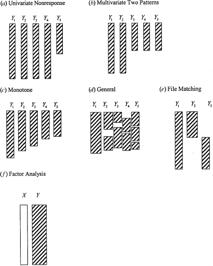
EXAMPLE 1.2. Unit and Item Nonresponse in Surveys. Another common pattern is obtained when the single incomplete variable Y_K in Figure 1.1a is replaced by a set of variables Y_J+1, … , Y_K, all observed or missing on the same set of cases (see Figure 1.1b, where K = 5 and J = 2). An example of this pattern is unit nonresponse in sample surveys, where a questionnaire is administered and a subset of sampled individuals do not complete the questionnaire because of noncontact, refusal, or some other reason. In that case the survey items are the incomplete variables, and the fully observed variables consist of survey design variables measured for respondents and nonrespondents, such as household location or characteristics measured in a listing operation prior to the survey. Common techniques for addressing unit nonresponse in surveys are discussed in Chapter 3. Survey practitioners call missing values on particular items in the questionnaire item nonresponse. These missing values typically have a haphazard pattern, such as that in Figure 1.1d. Item nonresponse in surveys is typically handled by imputation methods as discussed in Chapter 4, although the methods discussed in Part II of the book are also appropriate and relevant. For other discussions of missing data in the survey context, see Madow and Olkin (1983), Madow, Nisselson, and Olkin (1983), Madow, Olkin, and Rubin (1983), Rubin (1987a) and Groves et al. (2002).

EXAMPLE 1.3. Attrition in Longitudinal Studies. Longitudinal studies collect information on a set of cases repeatedly over time. A common missing-data problem is attrition, where subjects drop out prior to the end of the study and do not return. For example, in panel surveys members of the panel may drop out because they move to a location that is inaccessible to the researchers, or, in a clinical trial, some subjects drop out of the study for unknown reasons, possibly side effects of drugs, or curing of disease. The pattern of attrition is an example of monotone missing data, where the variables can be arranged so that all Y_j+1, … , Y_K are missing for cases where Y_j is missing, for all J = 1, … , K - 1 (see Figure 1.1c for K = 5). Methods for handling monotone missing data can be easier than methods for general patterns, as shown in Chapter 7 and elsewhere.

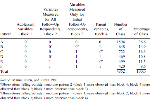
In practice, the pattern of missing data is rarely monotone, but is often close to monotone. Consider for example the data pattern in Table 1.1, which was obtained from the results of a panel study of students in 10 Illinois schools, analyzed by Marini, Olsen, and Rubin (1980). The first block of variables was recorded for all individuals at the start of the study, and hence is completely observed. The second block consists of variables measured for all respondents in the follow-up study, 15 years later. Of all respondents to the original survey, 79% responded to the follow-up, and thus the subset of variables in block 2 is regarded as 79% observed. Block 1 variables are consequently more observed than block 2 variables. The data for the 15-year follow-up survey were collected in several phases, and for economic reasons the group of variables forming the third block were recorded for a subset of those responding to block 2 variables. Thus, block 2 variables are more observed than block 3 variables. Blocks 1, 2, and 3 form a monotone pattern of missing data. The fourth block of variables consists of a small number of items measured by a questionnaire mailed to the parents of all students in the original adolescent sample. Of these parents, 65% responded. The four blocks of variables do not form a monotone pattern. However, by sacrificing a relatively small amount of data, monotone patterns can be obtained. The authors analyzed two monotone data sets. First, the values of block 4 variables for patterns C and E (marked with the letter b) are omitted, leaving a monotone pattern with block 1 more observed than block 2, which is more observed than block 3, which is more observed than block 4. Second, the values of block 2 variables for patterns B and D and the values of block 3 variables for pattern B (marked with the letter a) are omitted, leaving a monotone pattern with block 1 more observed than block 4, which is more observed than block 2, which is more observed than block 3. In other examples (such as the data in Table 1.2, discussed in Example 1.6 below), the creation of a monotone pattern involves the loss of a substantial amount of information.

Table 1.1 Patterns of Missing Data across Four Blocks of Variables: 0 = observed, 1 = missing).

Example 1.4. The File-Matching Problem, with Two Sets of Variables Never Jointly Observed. With large amounts of missing data, the possibility that variables are never observed together arises. When this happens, it is important to be aware of the problem since it implies that some parameters relating to the association between these variables are not estimable from the data, and attempts to estimate them may yield misleading results. Figure 1.1e illustrates an extreme version of this problem that arises in the context of combining data from two sources. In this pattern, Y₁ represents a set of variables that is common to both data sources and fully-observed, Y₂ a set of variables observed for the first data source but not the second, and Y₃ a set of variables observed for the second data source but not the first. Clearly there is no information in this data pattern about the partial associations of Y₂ and Y₃ given Y₁, in practice, analyses of data with this pattern typically make the strong assumption that these partial associations are zero. This pattern is discussed further in Section 7.5.

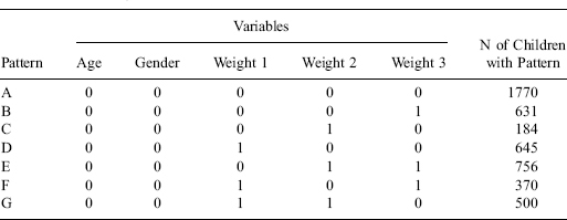
Table 1.2 Data Matrix for Children in a Survey Summarized by the Pattern of Missing Data: 0 = observed, 1 = missing.

Example 1.5. Latent-Variable Patterns with Variables that are Never Observed. It can be useful to regard certain problems involving unobserved “latent” variables as missing-data problems where the latent variables are completely missing, and then apply ideas from missing-data theory to estimate the parameters. Consider, for example, Figure 1.1f, where X represents a set of latent variables that are completely missing, and Y a set of variables that are fully observed. Factor analysis can be viewed as an analysis of the multivariate regression of Y on X for this pattern—that is, a pattern with none of the regressor variables observed! Clearly, some assumptions are needed. Standard forms of factor analysis assume the conditional independence of the components of Y given X . Estimation can be achieved by treating the factors X as missing data. If values of Y are also missing according to a haphazard pattern, then methods of estimation can be developed that treat both X and the missing values of Y as missing. This example is examined in more detail in Section 11.3.

Assumption 1.1: missingness indicators hide true values that are meaningful for analysis.

Assumption 1.1 may seem innocuous, but it has important implications for the analysis. When the assumption applies, it makes sense to consider analyses that effectively predict, or “impute” (that is, fill in) the unobserved values. If, on the other hand, Assumption 1.1 does not apply, then imputing the unobserved values makes little sense, and an analysis that creates strata of the population defined by the missingness indicator is more appropriate. Example 1.6 describes a situation with longitudinal data on obesity where Assumption 1.1 clearly makes sense. Example 1.7 describes the case of a randomized experiment where it makes sense for one outcome variable (survival) but not for another (quality of life). Example 1.8 describes a situation in opinion polling where Assumption 1.1 may or may not make sense, depending on the specific setting.

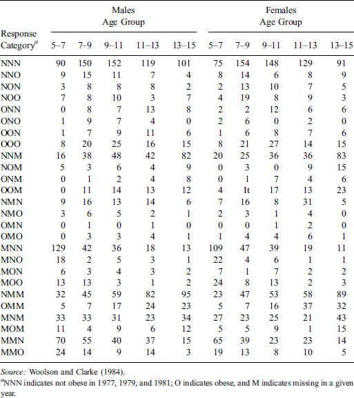
Example 1.6. Nonresponse in a Binary Outcome Measured at Three Time Points. Woolson and Clarke (1984) analyze data from the Muscatine Coronary Risk Factor Study, a longitudinal study of coronary risk factors in schoolchildren. Table 1.2 summarizes the data matrix by its pattern of missing data. Five variables (gender, age, and obesity for three rounds of the survey) are recorded for 4856 cases—gender and age are completely recorded, but the three obesity variables are sometimes missing with six patterns of missingness. Since age is recorded in five categories and the obesity variables are binary, the data can be displayed as counts in a contingency table. Table 1.3 displays the data in this form, with missingness of obesity treated as a third category of the variable, where O = obese, N = not obese, and M = missing. Thus the pattern MON denotes missing at the first round, obese at the second round, and not obese at the third round, and other patterns are defined similarly.

Woolson and Clarke analyze these data by fitting multinomial distributions over the 3³ - 1 = 26 response categories for each column in Table 1.3. That is, missingness is regarded as defining strata of the population. We suspect that for these data it makes good sense to regard the nonrespondents as having a true underlying value for the obesity variable. Hence we would argue for treating the nonresponse categories as missing value indicators and estimating the joint distribution of the three dichotomous outcome variables from the partially missing data. Appropriate methods for handling such categorical data with missing values effectively impute the values of obesity that are not observed, and are described in Chapter 12. The methods involve quite straightforward modifications of existing algorithms for categorical data analysis currently available in statistical software packages. For an analysis of these data that averages over patterns of missing data, see Ekholm and Skinner (1998).

Table 1.3 Number of Children Classified by Population and Relative Weight Category in Three Rounds of a Surve.

Example 1.7. Causal Effects of Treatments with Survival and Quality of Life Outcomes. Consider a randomized experiment with two drug treatment conditions, T = 0 or 1, and suppose that a primary outcome of the study is survival (D = 0) or death (D = 1) at one year after randomization to treatment. For participant i, let D_i(0) denote the one-year survival status if assigned treatment 0, and D_i(1) survival status if assigned treatment 1. The causal effect of treatment 1 relative to treatment 0 on survival for participant i is defined as D_i(1)- D_i(0). Estimation of this causal effect can be considered a missing-data problem, in that only one treatment can be assigned to each participant, so D_i(1) is unobserved (“missing”) for participants assigned treatment 0, and D_i(1) is unobserved (“missing”) for participants assigned treatment 1. Individual causal effects are unobserved, but randomization allows for unbiased estimation of average causal effects for a sample or population (Rubin, 1978a), which can be estimated from this missing-data perspective. The survival outcome under the treatment not received can be legitimately modeled as “missing data” in the sense of Assumption 1.1, since one can consider what the survival outcome would have been under the treatment not assigned, even though this outcome is never observed. For more applications of this “potential outcome” formulation to inference about causal effects, see, for example, Angrist, Imbens, and Rubin (1996), Barnard et al. (1998), Hirano et al. (2000), and Frangakis and Rubin (1999, 2001, 2002).

Rubin (2000) discusses the more complex situation where a “quality-of-life health indicator” Y (Y > 0) is also measured as a secondary outcome for those still alive one year after randomization to treatment. For participants who die within a year of randomization, Y is undefined in some sense or “censored” due to death—we think it usually makes little sense to treat these outcomes as missing values as in Assumption 1.1, given that quality of life is a meaningless concept for people who are not alive. More specifically, let D_i(T) denote the potential one-year survival outcome for participant i under treatment T , as before. The potential outcomes on D can be used to classify the patients into four groups:

1. Those who would live under either treatment assignment, LL = {i|D_i(0) = D_i(1) = 0}

2. Those who would die under either treatment assignment, DD = {i|D_i(0) = D_i(1) = 1}

3. Those who would live under control but die under treatment, LD = {i|D_i(0) = 0; D_i(1) = 1}

4. Those who would die under control but live under treatment DL = {i|D_i(0) = 1; D_i(1) = 0}

For the LL patients, there is a bivariate distribution of individual potential outcomes of Y under treatment and control, with one of these outcomes being observed and one missing. For the DD patients, there is no information on Y , and it is dubious to treat these values as missing. For LD patients there is a distribution of Y under the control condition, but not under the treatment condition, and for DL patients there is a distribution of Y under the new treatment condition but not under the control condition. Causal inference about Y can be conceptualized within this framework as imputing the survival status of participants under the treatment not received, and then imputing quality of life of participants under the treatment not received within the subpopulation of LL patients.

Example 1.8. Nonresponse in Opinion Polls. Consider the situation where individuals are polled about how they will vote in a future referendum, where the available responses are “yes,” “no,” or “missing.” Individuals who fail to respond to the question may be refusing to reveal real answers, or may have no interest in voting. Assumption 1.1 would not apply to individuals who would not vote, and these individuals define a stratum of the population that is not relevant to the outcome of the referendum. Assumption 1.1 would apply to individuals who do not respond to the initial poll but would vote in the referendum. For these individuals it makes sense to apply a method that effectively imputes a “yes” or “no” vote when analyzing the polling data. Rubin, Stern and Vehovar (1996) consider a situation where there is a complete list of eligible voters, and those who do not vote were counted as “no's” in the referendum. Here Assumption 1.1 applies to all the unobserved values in the initial poll. Consequently, Rubin, Stern and Vehovar (1996) consider methods that effectively impute the missing responses under a variety of modeling assumptions, as discussed in Example 15.14.

1.3. MECHANISMS THAT LEAD TO MISSING DATA

In the previous section we considered various patterns of missing data. A different issue concerns the mechanisms that lead to missing data, and in particular the question of whether the fact that variables are missing is related to the underlying values of the variables in the data set. Missing-data mechanisms are crucial since the properties of missing-data methods depend very strongly on the nature of the dependencies in these mechanisms. The crucial role of the mechanism in the analysis of data with missing values was largely ignored until the concept was formalized in the theory of Rubin (1976a), through the simple device of treating the missing-data indicators as random variables and assigning them a distribution. We now review this theory, using a notation and terminology that differs slightly from that of the original paper but has come into common use in the modern statistics literature on missing data.

Define the complete data Y = (y_ij) and the missing-data indicator matrix M = (M_ij) as in the previous section. The missing-data mechanism is characterized by the conditional distribution of M given Y , say f (M|Y , ϕ), where ϕ denotes unknown parameters. If missingness does not depend on the values of the data Y , missing or observed, that is, if

the data are called missing completely at random (MCAR)—note that this assumption does not mean that the pattern itself is random, but rather that missingness does not depend on the data values. Let Y_obs denote the observed components or entries of Y , and Y_mis the missing components. An assumption less restrictive than MCAR is that missingness depends only on the components Y_obs of Y that are observed, and not on the components that are missing. That is,

The missing-data mechanism is then called missing at random (MAR). The mechanism is called not missing at random (NMAR) if the distribution of M depends on the missing values in the data matrix Y .

Perhaps the simplest data structure is a univariate random sample for which some units are missing. Let Y = (y₁, … , y_n)^T where y_i denotes the value of a random variable for unit i, and let M = (M₁, … , M_n) where M_i = 0 for units that are observed and M_i = 1 for units that are missing. Suppose the joint distribution of (y_i, M_i) is independent across units, so in particular the probability that a unit is observed does not depend on the values of Y or M for other units. Then,

where f (y_i|θ) denotes the density of y_i indexed by unknown parameters θ, and f (M_i|y_i,θ) is the density of a Bernoulli distribution for the binary indicator M_i with probability Pr(M_i = 1| y_i, θ) that y_i is missing. If missingness is independent of Y , that is if Pr(M_i = 1|y_i, θ) = θ, a constant that does not depend on y_i, then the missing-data mechanism is MCAR (or in this case equivalently MAR). If the mechanism depends on y_i the mechanism is NMAR since it depends on y_i that are missing, assuming that there are some.

Let r denote the number of responding units (M_i = 0). An obvious consequence of the missing values in this example is the reduction in sample size from n to r. We might contemplate carrying out the same analyses on the reduced sample as we intended for the size-n sample. For example, if we assume the values are normally distributed and wish to make inferences about the mean, we might estimate the mean

by the sample mean of the responding units with standard error images

, where s is the sample standard deviation of the responding units. This strategy is valid if the mechanism is MCAR, since then the observed cases are a random subsample of all the cases. However, if the data are NMAR, the analysis based on the responding subsample is generally biased for the parameters of the distribution of Y .

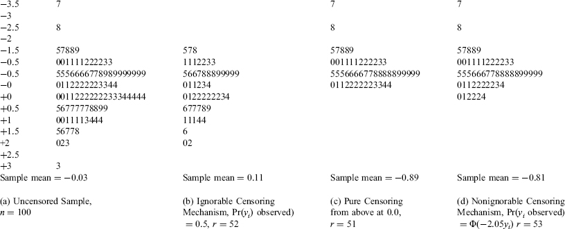
Example 1.9. Artificially-Created Missing Data in a Univariate Normal Sample. The data in Figure 1.2 provide a concrete illustration of this situation. Figure 1.2a presents a stem and leaf plot (i.e., a histogram with individual values retained) of n = 100 standard normal deviates. Under normality, the population mean (zero) for this sample is estimated by the sample mean, which has the value -0:03. Figure 1.2b presents a subsample of data obtained from the original sample in Figure 1.2a by deleting units by the MCAR mechanism:

independently with probability 0.5. The resulting sample of size r = 52 is a random subsample of the original values whose sample mean, -0:11, estimates the population mean of Y without bias.

Figures 1.2c and d illustrate NMAR mechanisms. In Figure 1.2c, negative values from the original sample have been retained and positive values have been deleted, that is,

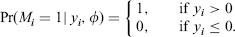
This mechanism is clearly NMAR, and the standard complete-data analysis that ignores the missing-data mechanism is biased. In particular, the sample mean, -0:89, obviously underestimates the population mean of Y. The mechanism (1.5) is a form of censoring, with observed values censored from above, or right censored, at the value zero.

where Φ(.) denotes the cumulative standard normal distribution function. The probability of being missing increases as y_i increases, and thus most of the observed values are negative. The missing-data mechanism is again NMAR, and the sample mean, -0:81 in the example, again systematically underestimates the population mean. The mechanism (1.6) is a form of stochastic censoring.

Now suppose that we are faced with an incomplete sample as in Figure 1.2c, and we wish to estimate the population mean. If the censoring mechanism is known, then methods are available that correct for the selection bias of the sample mean, as discussed in Section 15.3. If the censoring mechanism is unknown, the problem is much more difficult. The principal evidence that the response mechanism is not MAR lies in the fact that the observed samples are asymmetric, which contradicts the assumption that the original data have a (symmetric) normal distribution. If we are confident that the uncensored sample has a symmetric distribution, we can use this information to adjust for selection bias. On the other hand, if we have little knowledge about the form of the uncensored distribution, we cannot say whether the data are a censored sample from a symmetric distribution or a random subsample from an asymmetric distribution. In the former case, the sample mean is biased for the population mean; in the latter case it is not.

Figure 1.2. Stem and leaf displays of distribution of standard normal sample with stochastic censoring.

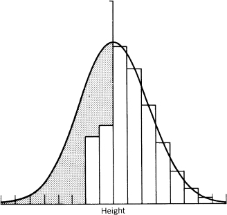
Example 1.10. Historical Heights. Wachter and Trussell (1982) present an interesting illustration of stochastic censoring, involving the estimation of historical heights. The distribution of heights in historical populations is of considerable interest in the biomedical and social sciences, because of the information it provides about nutrition, and hence indirectly about living standards. Most of the recorded information concerns the heights of recruits for the armed services. The samples are subject to censoring, since minimal height standards were often in operation and were enforced with variable strictness, depending on the demand for and supply of recruits. Thus a typical observed distribution of heights might take the form of the unshaded histogram in Figure 1.3, adapted from Wachter and Trussell, 1982. The shaded area in the figure represents the heights of men excluded from the recruit sample and is drawn under the assumption that heights are normally distributed in the uncensored population. Wachter and Trussell discuss methods for estimating the mean and variance of the uncensored distribution under this crucial normal assumption. In this example there is considerable external evidence that heights in unrestricted populations are nearly normal, so the inferences from the stochastically censored data under the assumption of normality have some validity. In many other problems involving missing data, such information is not available or is highly tenuous in nature. As discussed in Chapter 15, the sensitivity of answers from an incomplete sample to unjustifiable or tenuous assumptions is a basic problem in the analysis of data subject to unknown missing-data mechanisms, such as can occur in survey data subject to nonresponse.

Figure 1.3. Observed and population distributions of historical heights. Population distribution is normal, observed distribution is represented by the histogram, and the shaded area represents missing data.

Example 1.11. Mechanisms of Univariate Nonresponse (Example 1.1. continued). Suppose the data consist of an incomplete variable Y_K and a set of fully observed variables Y₁, … , Y_K-1, yielding the pattern of Figure 1.1a. As discussed in Examples 1.1 and 1.2, a wide variety of situations lead to the pattern in this figure. Since Y₁, … , Y_K-1 are fully observed, it is sufficient to define a single missing-data indicator variable M that takes the value 1 if Y_K is missing and 0 if Y_K is observed. Suppose that observations on Y and M are independent. The data are then MCAR if:

a constant that does not depend on any of the variables. The complete cases are then a random subsample of all the cases. The MCAR assumption is often too strong when the data on Y_K are missing because of uncontrolled events in the course of the data collection, such as nonresponse, or errors in recording the data, since these events are often associated with the study variables. The assumption may be more plausible if the missing data are missing by design. For example, if Y_K is the variable of interest but is expensive to measure, and Y₁, … , Y_K-1 are inexpensive surrogate measures for Y_K , then the pattern of Figure 1.1a can be obtained by a planned design where Y₁, … , Y_K-1 are recorded for a large sample and Y_K is recorded for a subsample. The technique of double sampling in survey methodology provides another instance of planned missing data. A large sample is selected, and certain basic characteristics are recorded. Then a random subsample is selected from the original sample, and more variables are measured. The resulting data form the pattern of this example, with Y_K replaced by a vector of measures (Fig. 1.1b).

so that missingness may depend on the fully observed variables Y₁, … , Y_K-1 but does not depend on the incomplete variable Y_K. If the probability that Y_K is missing depends on Y_K after conditioning on the other variables, then the mechanism is NMAR.

For example, suppose K = 2, Y₁ = age, and Y₂ = income. If the probability that income is missing is the same for all individuals, regardless of their age or income, then the data are MCAR. If the probability that income is missing varies according to the age of the respondent but does not vary according to the income of respondents with the same age, then the data are MAR. If the probability that income is recorded varies according to income for those with the same age, then the data are NMAR. This latter case is hardest to deal with analytically, which is unfortunate, since it may be the most likely case in this application. When missing data are not under control of the sampler, the MAR assumption is made more plausible by collecting data Y₁, … , Y_K-1 on respondents and nonrespondents that are predictive both of Y_K and the probability of being missing. Including these data in the analysis then reduces the association between M and Y_K, and helps to justify the MAR assumption. In the controlled missing-data environment of double sampling, the missing data are MAR, even if the probability of inclusion at the second stage is allowed to depend on the values of variables recorded at the first stage, a useful design strategy for improving efficiency in some applications.

The case of censoring illustrates a situation where the mechanism is NMAR but may be understood. The variable Y_K measures time to the occurrence of an event (e.g., death of an experimental animal, birth of a child, failure of a light bulb). For some units in the sample, time to occurrence is censored because the event had not occurred before the termination of data collection. If the time to censoring is known, then we have the partial information that the failure time exceeds the time to censoring. The analysis of the data needs to take account of this information to avoid biased conclusions.

The significance of these assumptions about the missing-data mechanism depends somewhat on the objective of the analysis. For example, if interest lies in the marginal distribution of Y₁, … , Y_K-1, then the data on Y_K , and the mechanism leading to missing values of Y_K , are usually irrelevant (“usually” because one can construct examples where this is not the case, but such examples are typically of theoretical rather than practical importance). If interest lies in the conditional distribution of Y_K given Y₁, … , Y_K-1, as, for example, when we are studying how the distribution of income varies according to age, and age is not missing, then the analysis based on the completely recorded units is satisfactory if the data are MAR. On the other hand, if interest is in the marginal distribution of Y_K (for example, summary measures such as the mean of Y_K), then an analysis based on the completely recorded units is generally biased unless the data are MCAR. With complete data on Y₁, … , Y_K-1 and Y_K, the data on Y₁, … , Y_K-1 are typically not useful in estimating the mean of Y_K , however, when data on Y_K are missing, the data on Y₁, … , Y_K-1 are useful for this purpose, both in increasing the efficiency with which the mean of Y_K is estimated and in reducing the effects of selection bias when the data are not MCAR. These points will be examined in more detail in subsequent chapters.

Example 1.12. Mechanisms of Attrition in Longitudinal Data (Example 1.3. continued). For the monotone pattern of attrition in longitudinal data (Fig. 1.1c for K = 5) the notation can again be simplified by defining a single missing indicator M that now takes the value j if Y₁, … , Y_j-1 are observed and Y_j , … , Y_K are missing (that is, dropout occurs between times (j - 1) and j, and the value K+ 1 for complete cases.) The missing data (dropout, attrition) mechanism is then MCAR if: