This text is printed on acid-free paper. 
Copyright © 1998 by John Wiley & Sons, Inc. All rights reserved.
Published simultaneously in Canada.
No part of this publication may be reproduced, stored in a retrieval system or transmitted in any form or by any means, electronic, mechanical, photocopying, recording, scanning or otherwise, except as permitted under Sections 107 or 108 of the 1976 United Stales Copyright Act, without either the prior written permission of the Publisher, or authorization through payment of the appropriate per-copy fee to the Copyright Clearance Center, 222 Rosewood Drive, Danvers. MA 01923, (978) 750-8400. fax (978) 750-4744. Requests to the Publisher for permission should be addressed to the Permissions Department, John Wiley & Sons, Inc., 605 Third Avenue. New York NY 10158-0012, (212) 850-60! I. fax (212) 850-6008. E-Mail: PERMREQ@WILFY.COM.
Library of Congress Cataloging-in-Publication Data:
Meeker. William Q.
Statistical methods for reliability data / William Q. Meeker. Luis A. Escobar.
p. cm. — (Wiley series in probability and statistics.
Applied probability and statistics)
“A Wiley-Interscience publication.”
Includes bibliographical references and index.
ISBN 0-471-14328-6 (cloth : alk. paper)
1. Reliability (Engineering)—Statistical methods. 1. Escobar.
Luis A. II. Title. III. Series.
TS173.M44 1998
620′.00452—dc21 97-39270
To Karen, Katherine, and my parents
W.Q.M.
To Lida, Juan, Catalina, Daniela, and my mother Inés
L.A.E.
Contents
Preface
Acknowledgments
1. Reliability Concepts and Reliability Data
1.1. Introduction
1.2. Examples of Reliability Data
1.3. General Models for Reliability Data
1.4. Repairable Systems and Nonrepairable Units
1.5. Strategy for Data Collection, Modeling, and Analysis
2. Models, Censoring, and Likelihood for Failure-Time Data
2.1. Models for Continuous Failure-Time Processes
2.2. Models for Discrete Data from a Continuous Process
2.3. Censoring
2.4. Likelihood
3. Nonparametric Estimation
3.1. Introduction
3.2. Estimation from Singly Censored Interval Data
3.3. Basic Ideas of Statistical Inference
3.4. Confidence Intervals from Complete or Singly Censored Data
3.5. Estimation from Multiply Censored Data
3.6. Pointwise Confidence Intervals from Multiply Censored Data
3.7. Estimation from Multiply Censored Data with Exact Failures
3.8. Simultaneous Confidence Bands
3.9. Uncertain Censoring Times
3.10. Arbitrary Censoring
4. Location-Scale-Based Parametric Distributions
4.1. Introduction.
4.2. Quantities of Interest in Reliability Applications
4.3. Location-Scale and Log-Location-Scale Distributions
4.4. Exponential Distribution
4.5. Normal Distribution
4.6. Lognormal Distribution
4.7. Smallest Extreme Value Distribution
4.8. Weibull Distribution
4.9. Largest Extreme Value Distribution
4.10. Logistic Distribution
4.11. Loglogistic Distribution
4.12. Parameters and Parameterization
4.13. Generating Pseudorandom Observations from a Specified Distribution
5. Other Parametric Distributions
5.1. Introduction
5.2. Gamma Distribution.
5.3. Generalized Gamma Distribution.
5.4. Extended Generalized Gamma Distribution
5.5. Generalized F Distribution
5.6. Inverse Gaussian Distribution
5.7. Birnbaum–Saunders Distribution
5.8. Gumpertz–Makeham Distribution
5.9. Comparison of Spread and Skewness Parameters
5.10. Distributions with a Threshold Parameter
5.11. Generalized Threshold-Scale Distribution
5.12. Other Methods of Deriving Failure-Time Distributions
6. Probability Plotting
6.1. Introduction
6.2. Linearizing Location-Scale-Based Distributions
6.3. Graphical Goodness of Fit.
6.4. Probability Plotting Positions
6.5. Probability Plots with Specified Shape Parameters.
6.6. Notes on the Application of Probability Plotting
7. Parametric Likelihood Fitting Concepts: Exponential Distribution
7.1. Introduction
7.2. Parametric Likelihood
7.3. Confidence Intervals for θ
7.4. Confidence Intervals for Functions of θ
7.5. Comparison of Confidence Interval Procedures
7.6. Likelihood for Exact Failure Times
7.7. Data Analysis with No Failures
8. Maximum Likelihood for Log-Location-Scale Distributions
8.1. Introduction
8.2. Likelihood
8.3. Likelihood Confidence Regions and Intervals
8.4. Normal-Approximation Confidence Intervals
8.5. Estimation with Given σ
9. Bootstrap Confidence Intervals
9.1. Introduction
9.2. Bootstrap Sampling
9.3. Exponential Distribution Confidence Intervals
9.4. Weibull, Lognormal, and Loglogistic Distribution Confidence Intervals
9.5. Nonparametric Bootstrap Confidence Intervals
9.6. Percentile Bootstrap Method
10. Planning Life Tests
10.1. Introduction
10.2. Approximate Variance of ML Estimators
10.3. Sample Size for Unrestricted Functions
10.4. Sample Size for Positive Functions
10.5. Sample Sizes for Log-Location-Scale Distributions with Censoring
10.6. Test Plans to Demonstrate Conformance with a Reliability Standard
10.7. Some Extensions
11. Parametric Maximum Likelihood: Other Models
11.1. Introduction
11.2. Fitting the Gamma Distribution
11.3. Fitting the Extended Generalized Gamma Distribution
11.4. Fitting the BISA and IGAU Distributions
11.5. Fitting a Limited Failure Population Model
11.6. Truncated Data and Truncated Distributions
11.7. Fitting Distributions that Have a Threshold Parameter
12. Prediction of Future Random Quantities
12.1. Introduction
12.2. Probability Prediction Intervals (θ Given)
12.3. Statistical Prediction Interval (θ Estimated)
12.4. The (Approximate) Pivotal Method for Prediction Intervals
12.5. Prediction in Simple Cases
12.6. Calibrating Naive Statistical Prediction Bounds
12.7. Prediction of Future Failures from a Single Group of Units in the Field
12.8. Prediction of Future Failures from Multiple Groups of Units with Staggered Entry into the Field
13. Degradation Data, Models, and Data Analysis
13.1. Introduction
13.2. Models for Degradation Data
13.3. Estimation of Degradation Model Parameters
13.4. Models Relating Degradation and Failure
13.5. Evaluation of F(t)
13.6. Estimation of F(r)y
13.7. Bootstrap Confidence Intervals
13.8. Comparison with Traditional Failure-Time Analyses
13.9. Approximate Degradation Analysis
14. Introduction to the Use of Bayesian Methods for Reliability Data
14.1. Introduction
14.2. Using Bayes’s Rule to Update Prior Information
14.3. Prior Information and Distributions
14.4. Numerical Methods for Combining Prior Information with a Likelihood
14.5. Using the Posterior Distribution for Estimation
14.6. Bayesian Prediction
14.7. Practical Issues in the Application of Bayesian Methods
15. System Reliability Concepts and Methods
15.1. Introduction
15.2. System Structures and System Failure Probability
15.3. Estimating System Reliability from Component Data
15.4. Estimating Reliability with Two or More Causes of Failure
15.5. Other Topics in System Reliability
16. Analysis of Repairable System and Other Recurrence Data
16.1. Introduction
16.2. Nonparametric Estimation of the MCF
16.3. Nonparametric Comparison of Two Samples of Recurrence Data
16.4. Parametric Models for Recurrence Data
16.5. Tools for Checking Point-Process Assumptions
16.6. Maximum Likelihood Fitting of Poisson Process
16.7. Generating Pseudorandom Realizations from an NHPP Process
16.8. Software Reliability
17. Failure-Time Regression Analysis
17.1. Introduction
17.2. Failure-Time Regression Models
17.3. Simple Linear Regression Models
17.4. Standard Errors and Confidence Intervals for Regression Models
17.5. Regression Model with Quadratic μ and Nonconstant σ
17.6. Checking Model Assumptions
17.7. Models with Two or More Explanatory Variables
17.8. Product Comparison: An Indicator-Variable Regression Model
17.9. The Proportional Hazards Failure-Time Model
17.10. General Time Transformation Functions
18. Accelerated Test Models
18.1. Introduction
18.2. Use-Rate Acceleration
18.3. Temperature Acceleration
18.4. Voltage and Voltage-Stress Acceleration
18.5. Acceleration Models with More than One Accelerating Variable
18.6. Guidelines for the Use of Acceleration Models
19. Accelerated Life Tests
19.1. Introduction
19.2. Analysis of Single-Variable ALT Data
19.3. Further Examples
19.4. Some Practical Suggestions for Drawing Conclusions from ALT Data
19.5. Other Kinds of Accelerated Tests
19.6. Potential Pitfalls of Accelerated Life Testing
20. Planning Accelerated Life Tests
20.1. Introduction
20.2. Evaluation of Test Plans
20.3. Planning Single-Variable ALT Experiments
20.4. Planning Two-Variable ALT Experiments
20.5. Planning ALT Experiments with More than Two Experimental Variables
21. Accelerated Degradation Tests
21.1. Introduction
21.2. Models for Accelerated Degradation Test Data
21.3. Estimating Accelerated Degradation Test Model Parameters
21.4. Estimation of Failure Probabilities, Distribution Quantiles, and Other Functions of Model Parameters
21.5. Confidence Intervals Based on Bootstrap Samples
21.6. Comparison with Traditional Accelerated Life Test Methods
21.7. Approximate Accelerated Degradation Analysis.
22. Case Studies and Further Applications
22.1. Dangers of Censoring in a Mixed Population
22.2. Using Prior Information in Accelerated Testing
22.3. An LFP/Competing Risk Model
22.4. Fatigue-Limit Regression Model
22.5. Planning Accelerated Degradation Tests
Epilogue
Appendix A. Notation and Acronyms
Appendix B. Some Results from Statistical Theory
B.1. cdfs and pdfs of Functions of Random Variables
B.2. Statistical Error Propagation—The Delta Method
B.3. Likelihood and Fisher Information Matrices
B.4. Regularity Conditions
B.5. Convergence in Distribution
B.6. Outline of General ML Theory
Appendix C. Tables
References
Author Index
Subject Index
Preface
Over the past 10 years there has been a heightened interest in improving quality, productivity, and reliability of manufactured products. Global competition and higher customer expectations for safe, reliable products are driving this interest. To meet this need, many companies have trained their design engineers and manufacturing engineers in the appropriate use of designed experiments and statistical process monitoring/control. Now reliability is being viewed as the product feature that has the potential to provide an important competitive edge. A current industry concern is in developing better processes to move rapidly from product conceptualization to a cost-effective highly reliable product. A reputation for unreliability can doom a product, if not the manufacturing company.
Data collection, data analysis, and data interpretation methods are important tools for those who are responsible for product reliability and product design decisions. This book describes and illustrates the use of proven traditional techniques for reliability data analysis and test planning, enhanced and brought up to date with modern computer-based graphical, analytical, and simulation-based methods. The material in this book is based on our interactions with engineers and statisticians in industry as well as on courses in applied reliability data analysis that we have taught to MS-level statistics and engineering students at both Iowa State University and Louisiana State University.
We have designed this book to be useful to statisticians and engineers working in industry as well as to students in university engineering and statistics programs. The book will be useful for on-the-job training courses in reliability data analysis. There is challenge in addressing such a wide-ranging audience. Communications among engineers and statisticians, however, is not only necessary but essential in the industrial research and development environment. We hope that this book will aid such communication. To produce a book that will appeal to both engineers and statisticians, we have placed primary focus on applications, data, concepts, methods, and interpretation. We use simple computational examples to illustrate ideas and concepts but, as in practical applications, rely on computers to do most of the computations. We have also included a collection of exercise problems at the end of each chapter. These exercises will give readers a chance to test their knowledge of basic material, to explore conceptual ideas of reliability testing, data analysis, and interpretation, and to see possible extensions of the material in the chapters.
It will be helpful for readers to have had a previous course in intermediate statistical methods covering basic ideas of statistical modeling and inference, graphical methods, estimation, confidence intervals, and regression analysis. Only the simplest concepts of calculus are used in the main body of the text (e.g., probability for a continuous random variable is computed as area under a density curve; a first derivative is a slope or a rate of change; a second derivative is a measure of curvature). Appendix B and some advanced exercises use calculus, linear algebra, basic optimization ideas, and basic statistical theory. Concepts, however, are presented in a relaxed and intuitive manner that we hope will also appeal to interested nonstatisticians. Throughout the book we have attempted to avoid the heavy language of mathematical statistics.
A detailed understanding of underlying statistical theory is not necessary to apply the methods in this book. Such details are, however, often important to understanding how to extend methods to new situations or developing new methods. Appendix B. at the end of the book, outlines the general theory and provides references to more detailed information. Also, many derivations and interesting extensions are covered in advanced guided exercises at the end of each chapter.
Particularly challenging exercises (i.e., exercises requiring knowledge of calculus or statistical theory) are marked with a triangle ( ). Exercises requiring computer programming (beyond the use of standard statistical packages) are marked with a diamond (
 ).
).
Special features of this book include the following:
The Wiley public ftp site includes special S-PLUS function examples created for the applications discussed in this book. The files can be accessed through either a standard ftp program or the ftp client of a Web browser using the http protocol. You can access the files from a Web browser through the following address:
http://www.wiley.com/products/subject/mathematics
On the Mathematics and Statistics home page you will see a link to the ftp Software Archive, which includes a link to information about the book and access to the software.
To gain ftp access, type the following at your Web browser’s URL address input box:
ftp://ftp.wiley.com
You can set an ID of anonymous; no password is required.
The files are located in the public/sci_tech_med/reliabilitv directory. Be sure to also download and read the README.TXT file, which includes directions on how to install and use the program.
If you need further information about downloading the files, you can reach Wiley’s tech support line at 212-850-6753.
Today there are many commercial statistical software packages. Unfortunately, only a few of these packages have adequate capabilities for doing reliability data analysis (e.g., the ability to do nonparametric and parametric estimation with censored data). Nelson (1990a, pages 237-240) outlines the capabilities of a number of commercial and noncommercial packages that were available at that time. As software vendors become more aware of their customers’ needs, capabilities in commercial packages are improving. Here we describe briefly the capabilities of a few packages that we and our colleagues have found to be useful.
MINITAB (1997), SAS PROC RELIABILITY (1997), SAS JMP (1995), S-PLUS (1996), and a specialized program called WinSMITH (Abemethy 1996) can do nonparametric and parametric product censored data analysis to estimate a single distribution (Chapters 3, 6, 7, and 8). SAS JMP can also analyze data with more than one failure mode (Chapter 15). MINITAB, SAS PROC RELIABILITY, SAS JMP, and S-PLUS can do parametric regression and accelerated life test analyses (Chapters 17 and 19), as well as semiparametric Cox proportional hazards regression analysis. SAS PROC RELIABILITY can, in addition, do the nonparametric repairable systems analyses (Chapter 16).
There are many possible paths that readers and instructors might take through this book. Chapters 1–16 cover single distribution models without any explanatory variables. Chapters 17–21 describe failure-time regression models. Chapter 22 presents case studies that illustrate, in the context of real problems, the integration of ideas presented throughout the book. This chapter also usefully illustrates how some of the general methods presented in the earlier chapters can be extended and adapted to deal with new problems.
Chapters 1–3 and 6–8 provide basic material that will be of interest to almost all readers and should be read in sequence. Chapter 4 discusses parametric failure-time models based on location-scale distributions and Chapter 5 covers more advanced distributional models. It is possible to use only a light reading of Chapter 4 and to skip Chapter 5 altogether before proceeding on to the important methods in Chapters 6–8. Chapter 9 explains and illustrates the use of bootstrap (simulation-based) methods for obtaining confidence intervals. Chapter 10 focuses on test planning: evaluating the effects of choosing sample size and length of observation. Chapters 11–16 cover a variety of special more advanced topics for single distribution models. Some of the material in Chapter 5 is prerequisite for the material in Chapter 11, but it is possible simply to work in Chapter 11, referring back to Chapter 5 only as needed. Otherwise, each of Chapters 10 through 14 has only material up to Chapter 8 as prerequisite. Chapter 15 introduces some important system reliability concepts and shows how the material in the first part of the book can be used to make statistical statements about the reliability of a system or a population of systems. Chapter 16 explains and illustrates the fundamental ideas behind analyzing system-repair and other recurrence data (as opposed to data on components and other replaceable units).
There are several groups of chapters on special topics that can be read in sequence.
Appendix A provides a summary and index of notation used in the book. Appendix B outlines the general maximum likelihood and other statistical theory on which the methods in the book are based. Appendix C gives tables for some of the larger data sets used in our examples.
A two-semester course would be required to cover thoroughly all of the material in the book. For a one-semester course, aimed at engineers and/or statisticians, an instructor could cover Chapters 1–4, 6–8, and 17–19, along with selected material from the appendices (according to the background of the students), and a few other chapters according to interests and tastes.
This book could be used as the basis for workshops or short courses aimed at engineers or statisticians working in industry. For an audience with a working knowledge of basic statistical tools, Chapters 1–3, key sections in Chapter 4. and Chapters 6–8 could be covered in one day. If the purpose of the short course is to introduce the basic ideas and illustrate with examples, then some material from Chapters 17–20 could also be covered. For a less experienced audience or for a more relaxed presentation, allowing time for exercises and discussion, two days would be needed to cover this material. Extending the course to three or four days would allow covering selected material in Chapters 9–22.
Ames, Iowa
Raton Rouge, Louisiana
April 1998
Acknowledgments
A number of individuals provided helpful comments on all or part of draft versions of this book. In particular, we would like to acknowledge Chuck Annis, Hwei-Chun Chou, William Christensen, Necip Doganaksoy, Tom Dubinin. Michael Eraas. Shuen-Lin Jeng, Gerry Hahn, Joseph Lu, Michael LuValle, Enid Martinets, Silvia Morales. Peter Morse, Dan Nordman, Steve Redman, Ernest Scheuer. Ananda Sen. David Steinberg, Mark Vandeven, Kim Wentzlaff, and a number of anonymous reviewers. Over the years, we have benefited from numerous technical discussions with Vijay Nair. Vijay provided a number of suggestions that substantially improved several parts of this book. We would also like to acknowledge our students (too numerous to mention by name) for their penetrating questions, high level of interest, and useful suggestions for improving our courses.
We would like to make special acknowledgment to Wayne Nelson, who gave us detailed feedback on earlier versions of most of the chapters of this book. Additionally, much of our knowledge in this area has it roots in our interactions with Wayne and Wayne’s outstanding books and other publications in the area of reliability and reliability data analysis.
Parts of this book were written while the first author was visiting the Department of Statistics and Actuarial Science at the University of Waterloo and the Department of Experimental Statistics at Louisiana State University. Support and use of facilities during these visits are gratefully acknowledged.
We greatly benefited from facilities, traveling support, and encouragement from Jeff Hooper and Michèle Boulanger at AT&T Bell Laboratories, Gerald Hahn at General Electric Corporate Research and Development Center, Enrique Villa and Victor Pérez Abreu at CIMAT in Guanajuato, México, Guido E. Del Pino at Universidad Católica in Santiago, Chile, Héctor Allende at Universidad Técnica Federico Santa María in Valparaiso, Chile, Yves L. Grize in Basel, Switzerland, and Stephan Zayac. Ford Motor Company.
Dean L. Isaacson, Head, Department of Statistics, Iowa State University, Lynn R. LaMotte, former Head, and E. Barry Moser, Interim Head, Department of Experimental Statistics, Louisiana State University, provided helpful encouragement and support to both authors. We would also like to thank our secretaries Denise Riker and Elaine Miller for excellent support and assistance while writing this book.
Finally, we would like to thank our wives and children for their love, patience, and understanding during the recent years in which we worked most weekends and many evenings to complete this project.
This chapter explains:
This chapter introduces some of the basic concepts of product reliability. Section 1.1 explains the relationship between quality and reliability and outlines how statistical studies are used to obtain information that can be used to assess and improve product reliability. Section 1.2 presents examples to illustrate studies that resulted in different kinds of reliability data. These examples are used in data analysis and exercises in subsequent chapters. Section 1.3 explains, in general terms, important qualitative aspects of statistical models that are used to describe populations and processes in reliability applications. Section 1.4 emphasizes the important distinction between studies focusing on data from repairable systems and nonrepairable units. Section 1.5 describes a general strategy for exploring, analyzing, and drawing conclusions from reliability data. This strategy is illustrated in examples throughout the book and in the case studies in Chapter 22.
Rapid advances in technology, development of highly sophisticated products, intense global competition, and increasing customer expectations have put new pressures on manufacturers to produce high-quality products. Customers expect purchased products to be reliable and safe. Systems, vehicles, machines, devices, and so on should, with high probability, be able to perform their intended function under usual operating conditions, for some specified period of time.
Technically, reliability is often defined as the probability that a system, vehicle, machine, device, and so on will perform its intended function under operating conditions, for a specified period of time. Improving reliability is an important part of (he larger overall picture of improving product quality. There are many definitions of quality, but general agreement that an unreliable product is not a high-quality product. Condra (1993) emphasizes that “reliability is quality over time.”
Modern programs for improving reliability of existing products and for assuring continued high reliability for the next generation of products require quantitative methods for predicting and assessing various aspects of product reliability. In most cases this will involve the collection of reliability data from studies such as laboratory tests (or designed experiments) of materials, devices, and components, tests on early prototype units, careful monitoring of early-production units in the field, analysis of warranty data, and systematic longer-term tracking of products in the field.
There are many possible reasons for collecting reliability data. Examples include the following:
Reliability data can have a number of special features requiring the use of special statistical methods. For example:
This book emphasizes the analysis of data from studies conducted to assess or improve product reliability. Data from reliability studies, however, closely resemble data from time-to-event studies in other areas of science and industry including biology, ecology, medicine, economics, and sociology. The methods of analysis in these other areas are the same or similar to those used in reliability data analysis. Some synonyms for reliability data are failure-time data, life data, survival data (used in medicine and biological sciences), and event-time data (used in the social sciences).
This section describes examples and data sets that illustrate the wide range of applications and characteristics of reliability data. These and other examples are used in subsequent chapters to illustrate the application of statistical methods for analyzing and drawing conclusions from such data.
In many applications reliability data will be collected on a sample of units that are assumed to have come from a particular process or population and to have been tested or operated under nominally identical conditions. More realistically, there are physical differences among units (e.g., strength or hardness) and operating conditions (e.g.. temperature, humidity, or stress) and these contribute to the variability in the data. The assumption used in drawing inferences from such single distribution data is that these differences accurately reflect the variability in life caused by the actual differences in the population or process of interest.
Example 1.1 Ball Bearing Fatigue Data. Lieblein and Zelen (1956) describe and give data from fatigue endurance tests for deep-groove ball bearings. The ball bearings came from four different major bearing companies. There was disagreement in the industry on the appropriate parameter values to use to describe the relationship between fatigue life and stress loading. The main objective of the study was to estimate values of the parameters in the equation relating bearing life to load.
The data shown in Table 1.1 are a subset of n = 23 bearing failure times for units tested at one level of stress, reported and analyzed by Lawless (1982). Figure 1.1 shows that the data are skewed to the right. Because of the lower bound on cycles (or time) to failure at zero, this distribution shape is typical of reliability data. Figure 1.2 illustrates the failure pattern over time.

Modern electronic systems may contain anywhere from hundreds to hundreds of thousands of integrated circuits (ICs). In order for such a system to have high reliability, it is necessary for the individual ICs and other components to have extremely high reliability, as in the following example.
Example 1.2 Integrated Circuit Life Test Data. Meeker (1987) reports the results of a life test of n = 4156 integrated circuits tested for 1370 hours at accelerated conditions of 80°C and 80% relative humidity. The accelerated conditions were used to shorten the test by causing defective units to fail more rapidly. The primary purpose of the experiment was to estimate the proportion of defective units being manufactured in the current production process and to estimate the amount of “burn-in” time that would be required to remove most of the defective units from the product population. The reliability engineers were also interested in whether it might be possible to get the needed information about the state of the production process, in the future, using much shorter tests (say, 200 or 300 hours). The data are reproduced in Table 1.2. There were 25 failures in the first 100 hours, three more between 100 and 600 hours, and no more failures out to 1370 hours, when the test was terminated. Ties in the data indicate that failures were detected at inspection times. A subset of the data is depicted in Figure 1.3.
Table 1.1. Ball Bearing Failure Times in Millions of Revolutions
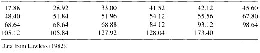
Figure 1.1. Histogram of the ball bearing failure data.
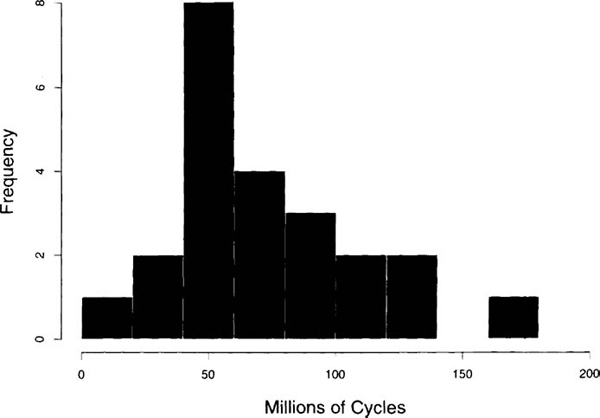
Figure 1.2. Display of the ball hearing failure data.
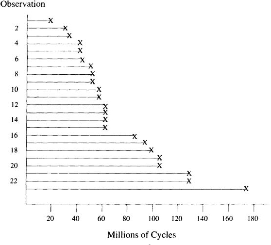
Table 1.2. Integrated Circuit Failure Times in Hours
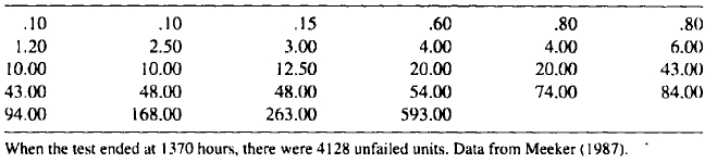
Figure 1.3. General failure pattern of the integrated circuit life test, showing a subset of the data where 28 out of 4156 units failed in the 1370-hour test
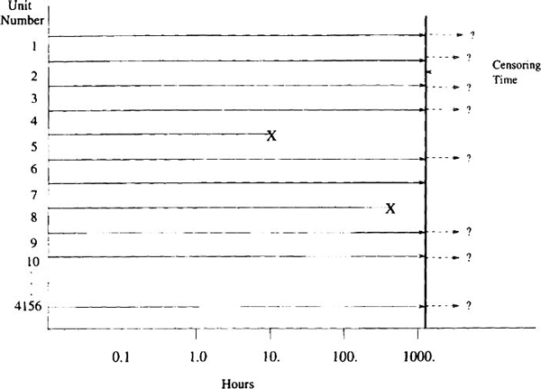
Table 1.3. Failure Data from a Circuit Pack Field Tracking Study
Example 1.3 Circuit Pack Reliability Field Trial. Table 1.3 gives information on the number of failures observed during periodic inspections in a field trial of early-production circuit packs employing new technology devices. The circuit packs were manufactured under the same design, but by two different vendors. The trial ran for 10,000 hours. The 4993 circuit packs from Vendor I came straight from production. The 4993 circuit packs from Vendor 2 had already seen 1000 hours of burn-in testing at the manufacturing plant under operating conditions similar to those in the field trial. Such circuit packs were sold at a higher price because field reliability was supposed to have been improved by the burn-in screening of circuit packs containing defective components. Failures during the first 1000 hours of burn-in were not recorded. This is the reason for the unknown entries in the table and for having information out to 11,000 hours for Vendor 2. The data in Table 1.3 is for the first failure in a position; information on circuit packs replaced after initial failure in a position was not part of the study.
Inspections were costly and were spaced more closely at the beginning of the study because more failures were expected there. The early “infant mortality” failures were caused by component defects in a small proportion of the circuit packs. Such failures are typical for an immature product. For such products, burn-in of circuit packs can be used to weed out most of the packs with weak components. Such burn-in, however, is expensive, and one of the manufacturer’s goals was to develop robust design and manufacturing processes that would eliminate or reduce, as quickly as possible, the occurrence of such defects in future generations of similar products.
There were several goals for this study:
Example 1.4 Diesel Generator Fan Failure Data. Nelson (1982, page 133) gives data on diesel generator fan failures. Failures in 12 of 70 generator fans were reported at times ranging between 450 hours and 8750 hours. Of the 58 units that did not fail, the reported running times (i.e., censoring times) ranged between 460 and 11,500 hours. Different fans had different running times because units were introduced into service at different times and because their use-rates differed. The data are reproduced in Appendix Table C.1. Figure 1.4 provides an initial graphical representation of the data. Figure 1.5 shows the censoring data. The data were collected to answer questions like:
Example 1.5 Heat Exchanger Tube Crack Data. Nuclear power plants use heat exchangers to transfer energy from the reactor to steam turbines. A typical heat exchanger contains thousands of tubes through which steam flows continuously when the heat exchanger is in service. With age, heat exchanger tubes develop cracks, usually due to some combination of stress-corrosion and fatigue. A heat exchanger can continue to operate safely when the cracks are small. If cracks get large enough, however, leaks can develop, and these could lead to serious safety problems and expensive, unplanned plant shut-down time. To protect against having leaks, heat exchangers are taken out of service periodically so that its tubes (and other components) can be inspected with nondestructive evaluation techniques. At the end of each inspection period, tubes with detected cracks are plugged so that water will no longer pass through them. This reduces plant efficiency but extends the life of the expensive heat exchangers. With this in mind, heat exchangers are built with extra capacity and can remain in operation up until the point where a certain percentage (e.g., 5%) of the tubes have been plugged.
Figure 1.4. Histogram showing failure times (light shade) and running times (dark shade) for the diesel generator fan data
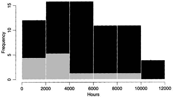
Figure 1.5. Failure pattern in a subset of the diesel generator fan data. There were 12 fan failures and 58 right-censored observations
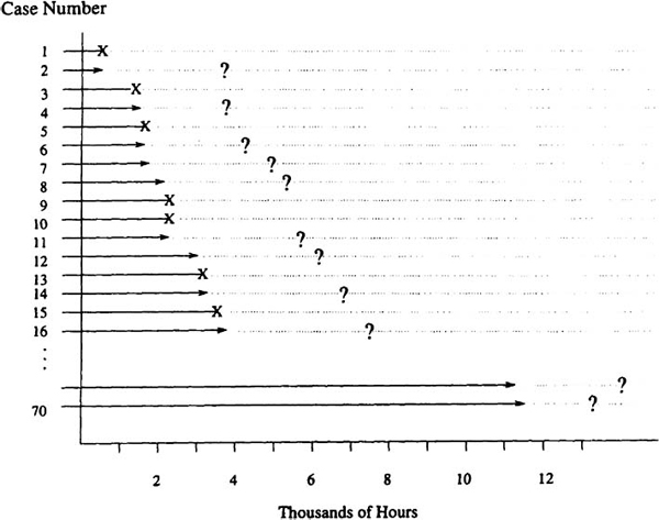
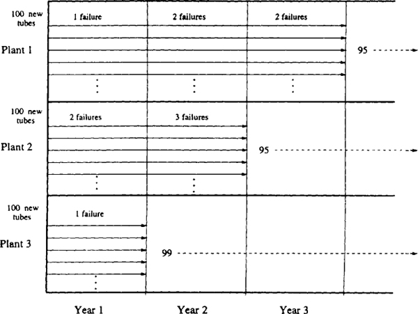
Figure 1.6 illustrates the inspection data, available at the end of 1983, from three different power plants. At this point in time, Plant 1 had been in operation for 3 years, Plant 2 for 2 years, and Plant 3 for only 1 year. Because all of the heat exchangers were manufactured according to the same design and specifications and because the heat exchangers were operated in generating plants run under similar tightly controlled conditions, it seemed that it should be reasonable to combine the data from the different plants for the sake of making inferences and predictions about the time-to-crack distribution of the heat exchanger tubes. Figure 1.7 illustrates the same data displayed in terms of amount of operating time instead of calendar time.
The engineers were interested in predicting tube life of a larger population of tubes in similar heat exchangers in other plants, for purposes of proper accounting and depreciation and so that the company could develop efficient inspection and replacement strategies. They also wanted to know if the tube failure rate was constant over time or if suspected wearout mechanisms (corrosion and fatigue) would, as suspected, begin to cause failures to occur with higher frequency as the heat exchanger ages.
Figure 1.6. Heat exchanger tube crack inspection data in calendar time.
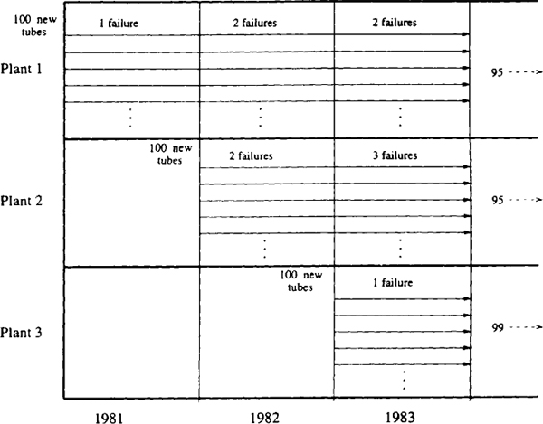
Figure 1.7. Heat exchanger tube crack inspection data in operating time
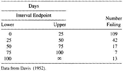
Example 1.6 Transmitter Vacuum Tube Data. Table 1.4 gives life data for a certain kind of transmitter vacuum tube (designated as “V7” within a particular transmitter design). Although solid-state electronics has made vacuum tubes obsolete for most applications, such tubes are still widely used in the output stage of high-power transmitters. These data were originally analyzed in Davis (1952). As seen in many practical situations, the exact failure times were not reported. Instead, we have only the number of failures in each interval or bin. Such data are known as grouped data, interval data, binned data, or read-out data.
Table 1.4. Failure Times for the V7 Transmitter Tlibe
Example 1.7 Turbine Wheel Crack Initiation Data. Nelson (1982) describes a study to estimate the distribution of time to crack initiation for turbine wheels. Each of 432 wheels was inspected once to determine if it had started to crack or not. At the time of the inspections, the wheels had different amounts of service time (age). A unit found to be cracked at its inspection was left-censored at its age (because the crack had initiated at some unknown point before its inspection age). A unit found to be uncracked at its inspection was right-censored at its age (because a crack would be initiated at some unknown point after that age). The data in Table 1.5, taken from Nelson (1982), show the number of cracked and uncracked wheels in different age categories, showing the midpoint of the time intervals given by Nelson. The data were put into intervals to facilitate simpler analyses.
In some applications components with an initiated crack could continue in service for rather long periods of time with the expectation that in-service inspections, scheduled frequently enough, could detect cracks before they grow to a size that could cause a safety hazard.
The important objectives of the study were to obtain information that could be used to:
Table 1.5. turbine Wheel Inspection Data Summary at Time of Study
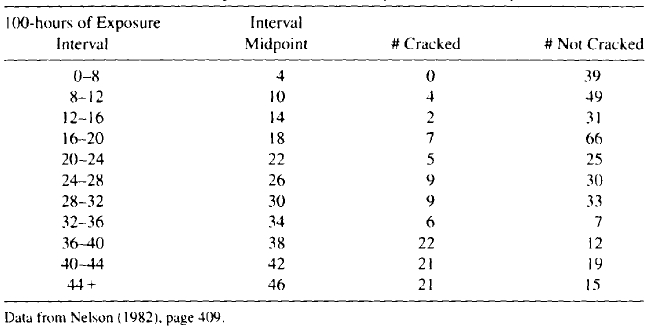
Figure 1.8. Turbine wheel inspection data summary at time of study
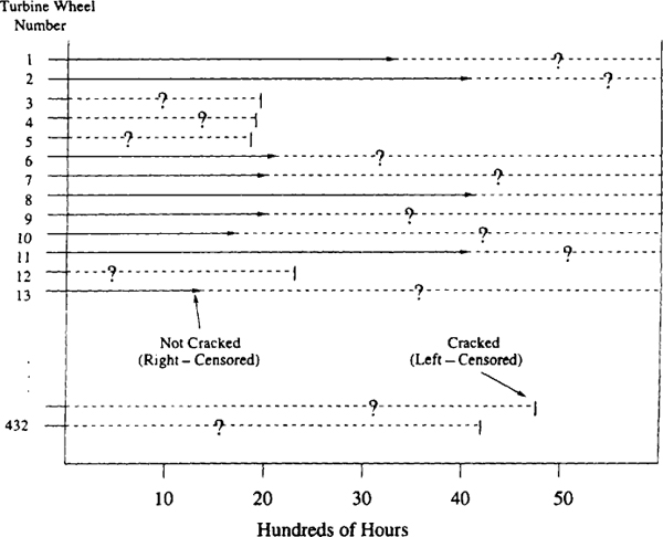
The failure/censoring pattern of these data is quite different from the previous examples and is illustrated in Figure 1.8. The analysts did not know the initiation time for any of the wheels. Instead, all they knew about each wheel was its age and whether a crack had initiated or not.
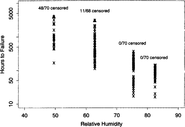
Example 1.8 Printed Circuit Board Accelerated Life Test Data. Meeker and LuValle (1995) give data from an accelerated life test on failure of printed circuit boards. The purpose of the experiment was to study the effect of the stresses on the failure-time distribution and to predict reliability under normal operating conditions. More specifically, the experiment was designed to study a particular failure mode—the formation and growth of conductive anodic filaments between copper-plated through-holes in the printed circuit boards. Actual growth of the filaments could not be monitored. Only failure time (defined as a short circuit) could be observed directly. Special test boards were constructed for the experiment. The data described here are part of the results of a much larger experiment aimed at determining the effects of temperature, relative humidity, and electric field on the reliability of printed circuit boards.
Figure 1.9. Scalier plot of printed circuit board accelerated life test data
Spacing between the holes in the test boards was chosen to simulate the spacing in actual printed circuit boards. Each test vehicle contained three identical 8 × 18 matrices of holes with alternate columns charged positively and negatively. These matrices, or “boards,” were the observational units in the experiment. Data analysis indicated that any clustering effect of boards within test boards was small enough to ignore in the study.
Meeker and LuValle (1995) give the number of failures that was observed in each of a series of 4-hour and 12-hour long intervals over the life test period. This experiment resulted in interval-censored data because only the interval in which each failure occurred was known. In this example all test units had the same inspection times. A graph of the data in Figure 1.9 plots the midpoint of the intervals containing failures versus relative humidity. The graph shows that failures occur earlier at higher levels of humidity.
Example 1.9 Accelerated Test of Spacecraft Nickel-Cadmium Battery Cells. Brown and Mains (1979) present the results of an extensive experiment to evaluate the long-term performance of rechargable nickel-cadmium battery cells that were to be used in spacecraft. The study used eight experimental factors. The first five factors shown in the table were environmental or accelerating factors (set to higher than usual levels to obtain failure information more quickly). The other three factors were product-design factors that could be adjusted in the product design to optimize performance and reliability of the batteries to be manufactured. The experiment ran 82 batteries, each containing 5 individual cells. Each battery was tested at a combination of factor levels determined according to a central composite experimental plan (see page 487 of Box and Draper, 1987, for information on central composite experimental designs).
Figure 1.10. Alloy-A fatigue crack size as a function of number of cycles
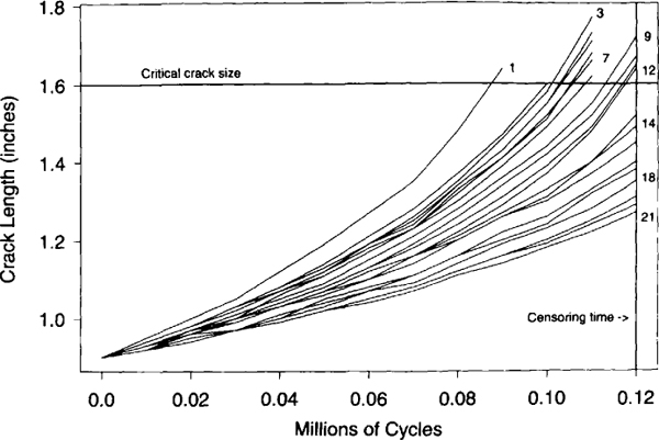
Example 1.10 Fatigue Crack-Size Data. Figure 1.10 and Appendix Table C.14 give the size of fatigue cracks as a function of number of cycles of applied stress for 21 test specimens. This is an example of degradation data. The data were reported originally in Hudak, Saxena, Bucci, and Malcolm (1978). The data were collected to obtain information on crack growth rates for the alloy. The data in Appendix Table C.14 were obtained visually from Figure 4.5.2 of Bogdanoff and Kozin (1985, page 242). For our analysis in the examples in Chapter 13, we will refer to these data as Alloy-A and assume that a crack of size 1.6 inches is considered to be a failure.