
Copyright © 2012 by John Wiley & Sons, Inc. All rights reserved
Published by John Wiley & Sons, Inc., Hoboken, New Jersey Published simultaneously in Canada
No part of this publication may be reproduced, stored in a retrieval system, or transmitted in any form or by any means, electronic, mechanical, photocopying, recording, scanning, or otherwise, except as permitted under Section 107 or 108 of the 1976 United States Copyright Act, without either the prior written permission of the Publisher, or authorization through payment of the appropriate per-copy fee to the Copyright Clearance Center, Inc., 222 Rosewood Drive, Danvers, MA 01923, (978) 750-8400, fax (978) 750-4470, or on the web at www.copyright.com. Requests to the Publisher for permission should be addressed to the Permissions Department, John Wiley & Sons, Inc., 111 River Street, Hoboken, NJ 07030, (201) 748-6011, fax (201) 748-6008, or online at http://www.wiley.com/go/permission.
Limit of Liability/Disclaimer of Warranty: While the publisher and author have used their best efforts in preparing this book, they make no representations or warranties with respect to the accuracy or completeness of the contents of this book and specifically disclaim any implied warranties of merchantability or fitness for a particular purpose. No warranty may be created or extended by sales representatives or written sales materials. The advice and strategies contained herein may not be suitable for your Situation. You should consult with a Professional where appropriate. Neither the publisher nor author shall be liable for any loss of profit or any other commercial damages, including but not limited to special, incidental, consequential, or other damages.
For general information on our other products and services or for technical support, please contact our Customer Care Department within the United States at (800) 762-2974, outside the United States at (317) 572-3993 or fax (317) 572-4002.
Wiley also publishes its books in a variety of electronic formats. Some content that appears in print may not be available in electronic formats. For more information about Wiley products, visit our web site at www.wiley.com.
Library of Congress Cataloging-in-Publication Data is available.
ISBN 978-1-118-31531-6
CONTENTS
1 INTRODUCTION
CHAPTER 2 SOLUTIONS
2.1 SECTION 2.2
CHAPTER 3 SOLUTIONS
3.1 SECTION 3.1
3.2 SECTION 3.2
3.3 SECTION 3.3
3.4 SECTION 3.4
3.5 SECTION 3.5
CHAPTER 4 SOLUTIONS
4.1 SECTION 4.2
CHAPTER 5 SOLUTIONS
5.1 SECTION 5.2
5.2 SECTION 5.3
5.3 SECTION 5.4
CHAPTER 6 SOLUTIONS
6.1 SECTION 6.1
6.2 SECTION 6.5
6.3 SECTION 6.6
CHAPTER 7 SOLUTIONS
7.1 SECTION 7,1
7.2 SECTION 7.2
7.3 SECTION 7.3
7.4 SECTION 7.5
CHAPTER 8 SOLUTIONS
8.1 SECTION 8.2
8.2 SECTION 8.3
8.3 SECTION 8.4
8.4 SECTION 8.5
8.5 SECTION 8.6
CHAPTER 9 SOLUTIONS
9.1 SECTION 9.1
9.2 SECTION 9.2
9.3 SECTION 9.3
9.4 SECTION 9.4
9.5 SECTION 9.6
9.6 SECTION 9.7
9.7 SECTION 9.8
CHAPTER 10 SOLUTIONS
10.1 SECTION 10.2
10.2 SECTION 10.3
10.3 SECTION 10.4
CHAPTER 11 SOLUTIONS
11.1 SECTION 11.2
11.2 SECTION 11.3
CHAPTER 12 SOLUTIONS
12.1 SECTION 12.1
12.2 SECTION 12.2
12.3 SECTION 12.3
12.4 SECTION 12.4
CHAPTER 13 SOLUTIONS
13.1 SECTION 13.1
13.2 SECTION 13.2
13.3 SECTION 13.3
13.4 SECTION 13.4
13.5 SECTION 13.5
CHAPTER 14
14.1 SECTION 14.7
CHAPTER 15
15.1 SECTION 15.2
15.2 SECTION 15.3
CHAPTER 16 SOLUTIONS
16.1 SECTION 16.3
16.2 SECTION 16.4
16.3 SECTION 16.5
CHAPTER 17 SOLUTIONS
17.1 SECTION 17.7
CHAPTER 18
18.1 SECTION 18.9
CHAPTER 19
19.1 SECTION 19.5
CHAPTER 20 SOLUTIONS
20.1 SECTION 20.1
20.2 SECTION 20.2
20.3 SECTION 20.3
20.4 SECTION 20.4
Established by WALTER A. SHEWHART and SAMUEL S. WILKS
Editors: David J. Baiding, NoelA. C. Cressie, Garrett M. Fitzmaurice, Harvey Goldstein, Iain M. Johnstone, Geert Molenberghs, David W. Scott, Adrian F. M. Smith, Ruey S. Tsay, Sanford Weisberg
Editors Emeriti: Vic Barnett, J. Stuart Hunter, Joseph B. Kadane, Jozef L. Teugels
A complete list of the titles in this series appears at the end of this volume.
The solutions presented in this manual reflect the authors’ best attempt to provide insights and answers. While we have done our best to be complete and accurate, errors may occur and there may be more elegant solutions. Errata will be posted at the ftp site dedicated to the text and solutions manual: ftp://ftp.wiley.com/public/sci_tech_med/loss_models/
Should you find errors or would like to provide improved solutions, please send your comments to Stuart Klugman at sklugman@soa.org.
2.1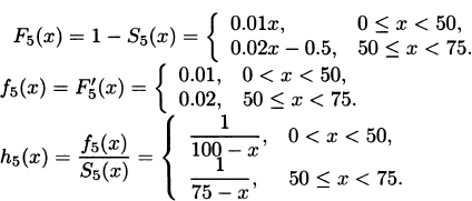
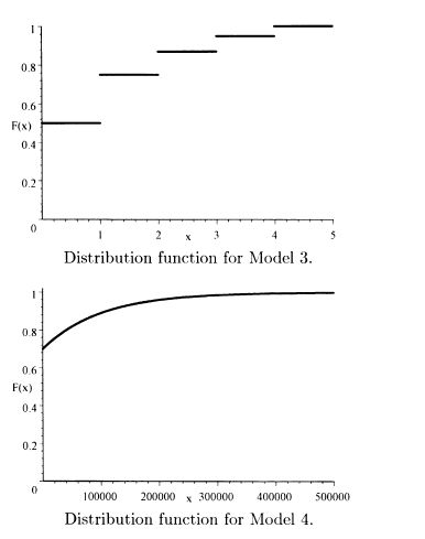
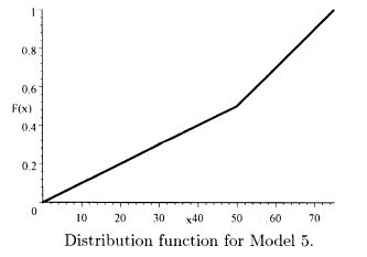
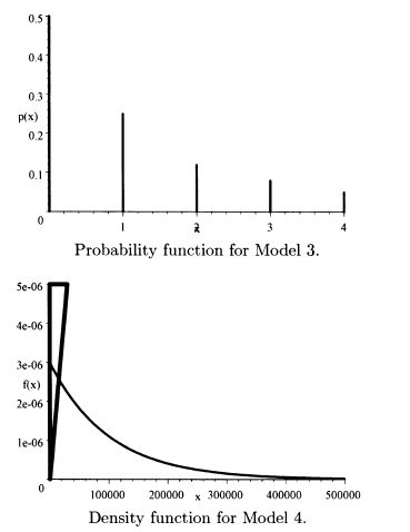
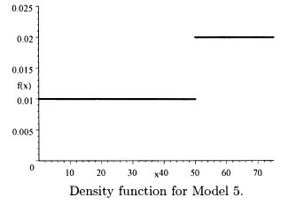
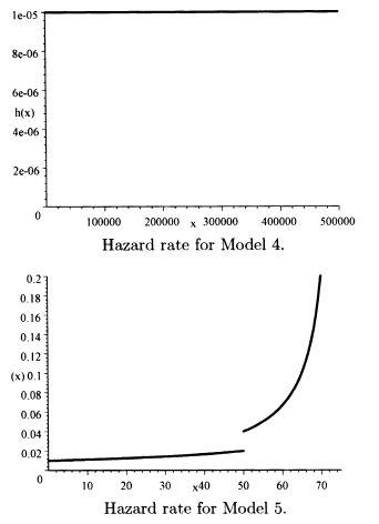
2.2 The requested plots follow. The triangular spike at zero in the density function for Model 4 indicates the 0.7 of discrete probability at zero.
2.3 f′(x) = 4(1 + x2)–3 – 24x2(l + x2)–4. Setting the derivative equal to zero and multiplying by (1 + x2)4 give the equation 4(1 + x2) – 24x2 = 0. This is equivalent to x2 = 1/5. The only positive solution is the mode of  .
.
2.4 The survival function can be recovered as

Taking logarithms gives

and thus A = 0.2009.
2.5 The ratio is
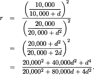
From observation or two applications of L’Hôpital’s rule, we see that the limit is infinity.
3.1
3.2 For Model 1, σ2 = 3,333.33 – 502 = 833.33, σ = 28.8675.

For Model 2, σ2 = 4,000,000 – 1,0002 = 3,000,000, σ = 1,732.05.  and
and  are both infinite so the skewness and kurtosis are not defined.
For Model 3, σ2 = 2.25 – .932 = 1.3851, σ = 1.1769.

For Model 4, σ2 = 6,000,000,000 – 30,0002 = 5,100,000,000, σ = 71,414.

For Model 5, σ2 = 2,395.83 – 43.752 = 481.77, σ = 21.95.

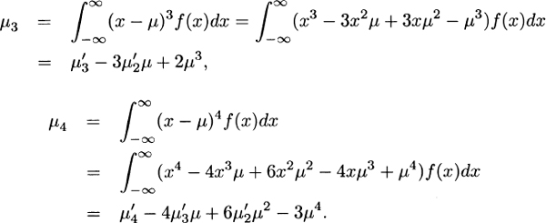
3.3 The Standard deviation is the mean times the coefficient, of Variation, or 4, and so the variance is 16. From (3.3) the second raw moment is 16 + 22 = 20. The third central moment is (using Exercise 3.1) 136 – 3(20)(2) + 2(2)3 = 32. The skewness is the third central moment divided by the cube of the Standard deviation, or 32/43 = 1/2.
3.4 For a gamma distribution the mean is αθ. The second raw moment is α(α + 1)θ2, and so the variance is αθ2. The coefficient of Variation is  /αθ = α–1/2 = 1. Therefore α = 1. The third raw moment is α(α + 1)(α + 2)θ3 = 6θ3. From Exercise 3.1, the third central moment is 6θ3 – 3(2θ2)θ + 2θ3 = 2θ3 and the skewness is 2θ3/(θ2)3/2 = 2.
3.5 For Model 1,

For Model 2,

For Model 3,
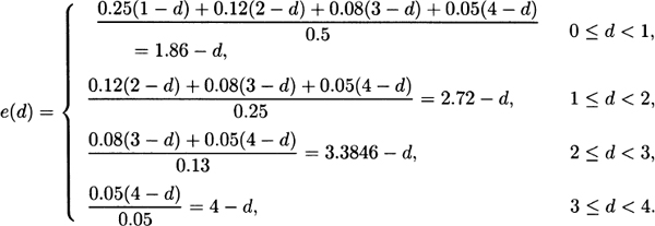
For Model 4,

The functions are straight lines for Models 1, 2, and 4. Model 1 has negative slope, Model 2 has positive slope, and Model 4 is horizontal.
3.6 For a uniform distribution on the interval from 0 to w, the density function is f(x) = 1/w. The mean residual life is
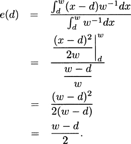
The equation becomes

with a solution of w = 108.
3.7 From the definition,

3.8

3.9 For Model 1, from (3.8),

and from (3.10),

From (3.9),

For Model 2, from (3.8),

and from (3.10),

From (3.9),

For Model 3, from (3.8),

and from (3.10),

For Model 4, from (3.8),

and from (3.10),

3.10 For a discrete distribution (which all empirical distributions are), the mean residual life function is

When d is equal to a possible value of X, the function cannot be continuous because there is jump in the denominator but not in the numerator. For an exponential distribution, argue as in Exercise 3.7 to see that it is constant. For the Pareto distribution,
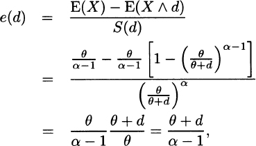
which is increasing in d. Only the second statement is true.
3.11 Applying the formula from the solution to Exercise 3.10 gives

which cannot be correct. Recall that the numerator of the mean residual life is E(X)–E(X  d). However, when α ≤ 1, the expected value is infinite and so is the mean residual life.
3.12 The right truncated variable is defined as Y = X given that X ≤ u. When X > u, this variable is not defined. The kth moment is

3.13 This is a single parameter Pareto distribution with parameters α = 2.5 and θ = 1. The moments are μ1 = 2.5/1.5 = 5/3 and μ2 = 2.5/.5 – (5/3)2 = 20/9. The coefficient of Variation is  /(5/3) = 0.89443.
3.14 μ = 0.05(100) + 0.2(200) + 0.5(300) + 0.2(400) + 0.05(500) = 300.
σ2 = 0.05(–200)2 + 0.2(–100)2 + 0.5(0)2 + 0.2(100)2 + 0.05(200)2 = 8,000.
μ3 = 0.05(–200)3 + 0.2(–100)3 + 0.5(0)3 + 0.2(100)3 + 0.05(200)3 = 0.
μ4 = 0.05(–200)4+0.2(–100)4+0.5(0)4+0.2(100)4+0.05(200)4 = 200,000,000.
Skewness is = γ1 = μ3/σ3 = 0. Kurtosis is γ2 = μ4/σ4 = 200,000,000/8,0002 = 3.125.
3.15 The Pareto mean residual life function is

and so eX (2θ)/eX(θ) = (2θ + θ)/(θ + θ) = 1.5.
3.16 Sample mean: 0.2(400) + 0.7(800) + 0.1(1,600) = 800. Sample variance: 0.2(–400)2 + 0.7(0)2 + 0.1(800)2 = 96,000. Sample third central moment: 0.2(–400)3 + 0.7(0)3 + 0.1 (800)3 = 38,400,000. Skewness coefficient: 38,400,000/96,0001.5 = 1.29.
3.17 The pdf is f(x) = 2x–3, x ≥ 1. The mean is  2x–2dx = 2. The median is the solution to .5 = F(x) = 1 – x–2, which is 1.4142. The mode is the value where the pdf is highest. Because the pdf is strictly decreasing, the mode is at its smallest value, 1.
3.18 For Model 2, solve  and so πp = 2,000[(1 – p)–1/3 – 1] and the requested percentiles are 519.84 and 1419.95.
For Model 4, the distribution function jumps from 0 to 0.7 at zero and so π0.5 = 0. For percentile above 70, solve p = 1 – 0.3e–0.00001πp, and so πp = –100,000 ln[(1 – p)/0.3] and π0.8 = 40,546.51.
For Model 5, the distribution function has two specifications. From x = 0 to x = 50 it rises from 0.0 to 0.5, and so for percentiles at 50 or below, the equation to solve is p = 0.01πp for πp = 100p. For 50 < x ≤ 75, the distribution function rises from 0.5 to 1.0, and so for percentiles from 50 to 100 the equation to solve is p = 0.02πp – 0.5 for πp = 50p + 25. The requested percentiles are 50 and 65.
3.19 The two percentiles imply
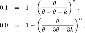
Rearranging the equations and taking their ratio yield

Taking logarithms of both sides gives ln 9 = α ln 3 for α = ln 9/ln 3 = 2.
3.20 The two percentiles imply

Subtracting and then taking logarithms of both sides give

Dividing the second equation by the first gives

Finally, taking logarithms of both sides gives τ ln 100 = ln[ln 0.25/ln 0.75] for τ = 0.3415.
3.21 The sum has a gamma distribution with parameters α = 16 and θ = 250. Then, Pr(S16 > 6,000) = 1 – Γ(16; 6,000/250) = 1 – Γ(16;24). From the Central Limit Theorem, the sum has an approximate normal distribution with mean αθ = 4,000 and variance αθ2 = 1,000,000 for a Standard deviation of 1000. The probability of exceeding 6,000 is 1 – Φ[(6,000 – 4,000)/1,000] = 1 – Φ(2) = 0.0228.
3.22 A single claim has mean 8,000/(5/3) = 4,800 and variance

The sum of 100 claims has mean 480,000 and variance 9,216,000,000, which is a Standard deviation of 96,000. The probability of exceeding 600,000 is approximately

3.23 The mean of the gamma distribution is 5(1,000) = 5,000 and the variance is 5(1,000)2 = 5,000,000. For 100 independent claims, the mean is 500,000 and the variance is 500,000,000 for a Standard deviation of 22,360.68. The probability of total claims exceeding 525,000 is

3.24 The sum of 2,500 contracts has an approximate normal distribution with mean 2,500(1,300) = 3,250,000 and Standard deviation  (400) = 20,000. The answer is Pr(X > 3,282,500)
  Pr[Z > (3,282,500 – 3,250,000)/20,000] = Pr(Z > 1.625) = 0.052.
3.25 While the Weibull distribution has all positive moments, for the inverse Weibull moments exist only for k < τ. Thus by this criterion, the inverse Weibull distribution has a heavier tail. With regard to the ratio of density functions, it is (with the inverse Weibull in the numerator and marking its Parameters with asterisks)

The logarithm is

The middle term goes to zero, so the issue is the limit of (x/θ)τ – (τ + τ*) ln x, which is clearly infinite. With regard to the hazard rate, for the Weibull distribution we have

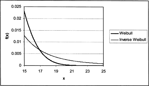
Figure 3.1 Tails of a Weibull and inverse Weibull distribution.
which is clearly increasing when τ > 1, constant when τ = 1, and decreasing when τ < 1. For the inverse Weibull,

The derivative of the denominator is

and the limiting value of this expression is θτ > 0. Therefore, in the limit, the denominator is increasing and thus the hazard rate is decreasing.
Figure 3.1 displays a portion of the density function for Weibull (τ = 3, θ = 10) and inverse Weibull (τ = 4.4744, θ = 7.4934) distributions with the same mean and variance. The heavier tail of the inverse Weibull distribution is clear.
3.26 Means:

Second moments:

Density functions:

The gamma and lognormal densities are equal when x = 2,221 while the lognormal and Pareto densities are equal when x = 9,678. Numerical evaluation indicates that the ordering is as expected.
3.27 For the Pareto distribution
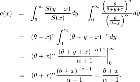
Thus e(x) is clearly increasing and e(x) ≥ 0, indicating a heavy tail.
The square of the coefficient of Variation is

which is greater than 1, also indicating a heavy tail.
3.28

This result assumes limy→∞ etySX(y) = 0. An application of L’Höpital’s rule shows that this is the saine limit as (–t–1) limy→∞ ety fX(y). This liniit must be zero, otherwise the integral defining MX(t) will not converge.
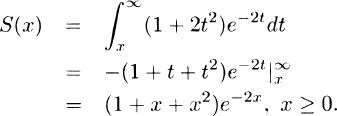
3.29 (a)
(b)

(c) For y ≥ 0,

Thus,

(d)

(e) Using (b),

(f) Using (d), we have

and so

Also, from (b) and (e), h(0) = 1,  , and h(∞) = 2.
3.30 (a) Integration by parts yields

and hence  , from which the result follows.
(b) It follows from (a) that

which gives the result by addition of xS(x) to both sides.
(c) Because e(x) = E(X)Se(x)/S(x), from (b)

and the first result follows by division of both sides by x + e(x). The inequality then follows from  .
.
(d) Because e(0) = E(X), the result follows from the inequality in (c) with e(x) replaced by E(X) in the denominator.
(e) As in (c), it follows from (b) that

that is,

from which the first result follows by solving for Se(x). The inequality then follows from the first result since  .
.
3.31 Denote the risk measures by ρ(X) = μX + kσX, ρ(Y) = μY + kσY and ρ(X + Y) = μX+Y + kσX+Y. Note that μX+Y = μX + μY and

where ρ here is the correlation coefficient, not the risk measure, and must be less than or equal to one. Therefore, σX+Y ≤ σX + σY. Thus,

which establishes subadditivity.
Because μcX = cμX and σcX = cσX, ρ(cX) = cμX + kcσX = cp(X), which establishes positive homogeneity.
Because μX+c = μX + c and σX+c = σX, ρ(X + c) = μX + c + kσX = ρ(X) + c, which establishes translation invariance.
For the example given, note that X ≤ Y for all possible pairs of outcomes. Also, μX = 3, μY = 4, σX =  , σY = 0. With k = 1, ρ(X) = 3 +
  4.732. which is greater than ρ(Y) = 4 + 0 = 4, violating monotonicity.
3.32 The cdf is F(x) = 1 – exp(–x/θ), and so the percentile solves p = 1 – exp(–πp/θ) and the solution is VaRp(X) = πp = –θ ln(1 – p). Because the exponential distribution is memoryless, e(πp) = θ and so TVaRp(X) =VaRp(X)+ e(πp) = πp + θ.
3.33 The cdf is F(x) = 1 – [θ/(θ + x)]α and so the percentile solves p = 1 – [θ/(θ + πp)]α and the solution is VaRp(X) = πp = θ[(1 – p)–1/α – 1]. From (3.13) and Appendix A,
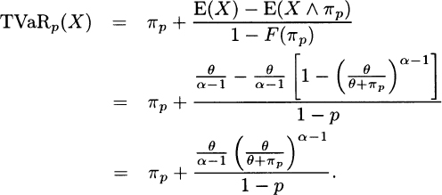
Substitute 1 – p for [θ/(θ + πp)]α to obtain

3.34 First, obtain

Using πp = μ + σΦ–1(p), the results for the normal distribution are obtained.
For the Pareto distribution, using θ = 150 and α = 2.5 and the formulas in Example 3.17,

will yield the results.
For the Weibull(50,0.5) distribution and the formulas in Appendix A,

from which

which gives the results.
3.35 From Exercise 3.34, VaR0.999(X) = π0.999 = 2,385.85. The mean is E(X) = θΓ(1 + 1/τ) = 50Γ(3) = 100. From Appendix A,

The value of Γ(3; 6.9078) can be obtained using the Excel function GAMMADIST(6.90775, 3, 1, TRUE). It is 0.968234.
Therefore, E(X  π0.999) = 99.209. From these results using (3.13),

(The answer is sensitive to the number of decimal places retained.)
3.36 For the exponential distribution,

Therefore TVaR0.95(X) = 1,997.866.
From Example 3.19, for the Pareto distribution,

3.37 For x > x0,
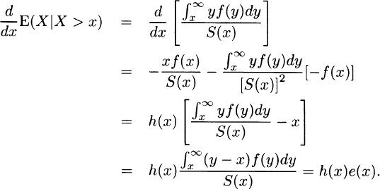
Because h(x) ≥ 0 and e(x) ≥ 0, the derivative must be nonnegative.
4.1 Arguing as in the examples,
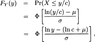
which indicates that Y has the lognormal distribution with parameters μ-ln c and σ Because no parameter was multiplied by c, there is no scale parameter. To introduce a scale parameter, define the lognormal distribution function as F(x) =  . Note that the new parameter v is simply eμ. Then, arguing as before,
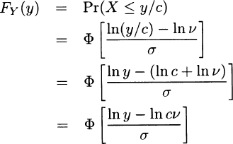
demonstrating that v is a scale parameter.
4.2 The following is not the only possible set of answers to this question. Model 1 is a uniform distribution on the interval 0 to 100 with parameters 0 and 100. It is also a beta distribution with parameters a = 1, b = 1, and θ = 100. Model 2 is a Pareto distribution with parameters α = 3 and θ = 2000. Model 3 would not normally be considered a parametric distribution. However, we could define a parametric discrete distribution with arbitrary probabilities at 0,1,2,3, and 4 being the parameters. Conventional usage would not accept this as a parametric distribution. Similarly, Model 4 is not a Standard parametric distribution, but we could define one as having arbitrary probability p at zero and an exponential distribution elsewhere. Model 5 could be from a parametric distribution with uniform probability from a to b and a different uniform probability from b to c.
4.3 For this year,

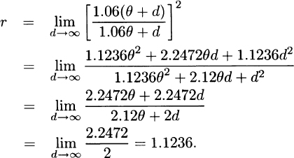
For next year, because θ is a scale parameter, claims will have a Pareto distribution with parameters α = 2 and 1.06θ. That makes the probability  . Then
4.4 The mth moment of a k-point mixture distribution is

For this problem, the first moment is

Similarly, the second moment is

4.5 Using the results from Exercise 4.4, E(X) = 


