Contents
Preface
1 The principles and limitations of geophysical exploration methods
1.1 Introduction
1.2 The survey methods
1.3 The problem of ambiguity in geophysical interpretation
1.4 The structure of the book
2 Geophysical data processing
2.1 Introduction
2.2 Digitization of geophysical data
2.3 Spectral analysis
2.4 Waveform processing
2.5 Digital filtering
2.6 Imaging and modelling
Further reading
3 Elements of seismic surveying
3.1 Introduction
3.2 Stress and strain
3.3 Seismic waves
3.4 Seismic wave velocities of rocks
3.5 Attenuation of seismic energy along ray paths
3.6 Ray paths in layered media
3.7 Reflection and refraction surveying
3.8 Seismic data acquisition systems
Further reading
4 Seismic reflection surveying
4.1 Introduction
4.2 Geometry of reflected ray paths
4.3 The reflection seismogram
4.4 Multichannel reflection survey design
4.5 Time corrections applied to seismic traces
4.6 Static correction
4.7 Velocity analysis
4.8 Filtering of seismic data
4.9 Migration of reflection data
4.10 3D seismic reflection surveys
4.11 Three component (3C) seismic reflection surveys
4.12 4D seismic reflection surveys
4.13 Vertical seismic profiling
4.14 Interpretation of seismic reflection data
4.15 Single-channel marine reflection profiling
4.16 Applications of seismic reflection surveying
Further reading
5 Seismic refraction surveying
5.1 Introduction
5.2 Geometry of refracted ray paths: planar interfaces
5.3 Profile geometries for studying planar layer problems
5.4 Geometry of refracted ray paths: irregular (non-planar) interfaces
5.5 Construction of wavefronts and ray-tracing
5.6 The hidden and blind layer problems
5.7 Refraction in layers of continuous velocity change
5.8 Methodology of refraction profiling
5.9 Other methods of refraction surveying
5.10 Seismic tomography
5.11 Applications of seismic refraction surveying
Further reading
6 Gravity surveying
6.1 Introduction
6.2 Basic theory
6.3 Units of gravity
6.4 Measurement of gravity
6.5 Gravity anomalies
6.6 Gravity anomalies of simple-shaped bodies
6.7 Gravity surveying
6.8 Gravity reduction
6.9 Rock densities
6.10 Interpretation of gravity anomalies
6.11 Elementary potential theory and potential field manipulation
6.12 Applications of gravity surveying
Further reading
7 Magnetic surveying
7.1 Introduction
7.2 Basic concepts
7.3 Rock magnetism
7.4 The geomagnetic field
7.5 Magnetic anomalies
7.6 Magnetic surveying instruments
7.7 Ground magnetic surveys
7.8 Aeromagnetic and marine surveys
7.9 Reduction of magnetic observations
7.10 Interpretation of magnetic anomalies
7.11 Potential field transformations
7.12 Applications of magnetic surveying
Further reading
8 Electrical surveying
8.1 Introduction
8.2 Resistivity method
8.3 Induced polarization (IP) method
8.4 Self-potential (SP) method
Further reading
9 Electromagnetic surveying
9.1 Introduction
9.2 Depth of penetration of electromagnetic fields
9.3 Detection of electromagnetic fields
9.4 Tilt-angle methods
9.5 Phase measuring systems
9.6 Time-domain electromagnetic surveying
9.7 Non-contacting conductivity measurement
9.8 Airborne electromagnetic surveying
9.9 Interpretation of electromagnetic data
9.10 Limitations of the electromagnetic method
9.11 Telluric and magnetotelluric field methods
9.12 Ground-penetrating radar
9.13 Applications of electromagnetic surveying
Further reading
10 Radiometric surveying
10.1 Introduction
10.2 Radioactive decay
10.3 Radioactive minerals
10.4 Instruments for measuring radioactivity
10.5 Field surveys
10.6 Example of radiometric surveying
Further reading
11 Geophysical borehole logging
11.1 Introduction to drilling
11.2 Principles of well logging
11.3 Formation evaluation
11.4 Resistivity logging
11.5 Induction logging
11.6 Self-potential logging
11.7 Radiometric logging
11.8 Sonic logging
11.9 Temperature logging
11.10 Magnetic logging
11.11 Gravity logging
Further reading
Appendix: SI, c.g.s. and Imperial (customary USA) units and conversion factors
References
Supplemental images
Index
© 2002 by
Blackwell Science Ltd
Editorial Offices:
Osney Mead, Oxford OX2 0EL
25 John Street, London WC1N 2BS
23 Ainslie Place, Edinburgh EH3 6AJ
350 Main Street, Malden
MA 02148-5018, USA
54 University Street, Carlton
Victoria 3053, Australia
10, rue Casimir Delavigne
75006 Paris, France
Other Editorial Offices:
Blackwell Wissenschafts-Verlag GmbH
Kurfürstendamm 57
10707 Berlin, Germany
Blackwell Science KK
MG Kodenmacho Building
7–10 Kodenmacho Nihombashi
Chuo-ku, Tokyo 104, Japan
Iowa State University Press
A Blackwell Science Company
2121 S. State Avenue
Ames, Iowa 50014-8300, USA
First published 1984
Reprinted 1987, 1989
Second edition 1991
Reprinted 1992, 1993, 1994, 1995, 1996 1998, 1999, 2000
Third edition 2002
Set by SNP Best-set Typesetter Ltd.,
Hong Kong
The right of the Authors to be identified as the Authors of this Work has been asserted in accordance with the Copyright, Designs and Patents Act 1988.
All rights reserved. No part of this publication may be reproduced, stored in a retrieval system, or transmitted, in any form or by any means, electronic, mechanical, photocopying, recording or otherwise, except as permitted by the UK Copyright, Designs and Patents Act 1988, without the prior permission of the copyright owner.
A catalogue record for this title is available from the British Library
ISBN 0-632-04929-4
Library of Congress
Cataloging-in-Publication Data has been applied for
The Blackwell Science logo is a trade mark of Blackwell Science Ltd, registered at the United Kingdom Trade Marks Registry
DISTRIBUTORS
Marston Book Services Ltd
PO Box 269
Abingdon, Oxon OX14 4YN
(Orders: Tel: 01235 465500 Fax: 01235 465555)
The Americas
Blackwell Publishing
c/o AIDC
PO Box 20
50 Winter Sport Lane
Williston, VT 05495-0020
(Orders: Tel: 800 216 2522 Fax: 802 864 7626)
Australia
Blackwell Science Pty Ltd
54 University Street
Carlton, Victoria 3053
(Orders: Tel: 3 9347 0300 Fax: 3 9347 5001)
For further information on
Blackwell Science, visit our website:
www.blackwell-science.com
Preface
This book provides a general introduction to the most important methods of geophysical exploration. These methods represent a primary tool for investigation of the subsurface and are applicable to a very wide range of problems. Although their main application is in prospecting for natural resources, the methods are also used, for example, as an aid to geological surveying, as a means of deriving information on the Earth’s internal physical properties, and in engineering or archaeological site investigations. Consequently, geophysical exploration is of importance not only to geophysicists but also to geologists, physicists, engineers and archaeologists. The book covers the physical principles, methodology, interpretational procedures and fields of application of the various survey methods. The main emphasis has been placed on seismic methods because these represent the most extensively used techniques, being routinely and widely employed by the oil industry in prospecting for hydrocarbons. Since this is an introductory text we have not attempted to be completely comprehensive in our coverage of the subject. Readers seeking further information on any of the survey methods described should refer to the more advanced texts listed at the end of each chapter.
We hope that the book will serve as an introductory course text for students in the above-mentioned disciplines and also as a useful guide for specialists who wish to be aware of the value of geophysical surveying to their own disciplines. In preparing a book for such a wide possible readership it is inevitable that problems arise concerning the level of mathematical treatment to be adopted. Geophysics is a highly mathematical subject and, although we have attempted to show that no great mathematical expertise is necessary for a broad understanding of geophysical surveying, a full appreciation of the more advanced data processing and interpretational techniques does require a reasonable mathematical ability. Our approach to this problem has been to keep the mathematics as simple as possible and to restrict full mathematical analysis to relatively simple cases. We consider it important, however, that any user of geophysical surveying should be aware of the more advanced techniques of analysing and interpreting geophysical data since these can greatly increase the amount of useful information obtained from the data. In discussing such techniques we have adopted a semiquantitative or qualitative approach which allows the reader to assess their scope and importance, without going into the details of their implementation.
Earlier editions of this book have come to be accepted as the standard geophysical exploration textbook by numerous higher educational institutions in Britain, North America, and many other countries. In the third edition, we have brought the content up to date by taking account of recent developments in all the main areas of geophysical exploration. We have extended the scope of the seismic chapters by including new material on three-component and 4D reflection seismology, and by providing a new section on seismic tomography. We have also widened the range of applications of refraction seismology considered, to include an account of engineering site investigation.
This chapter is provided for readers with no prior knowledge of geophysical exploration methods and is pitched at an elementary level. It may be passed over by readers already familiar with the basic principles and limitations of geophysical surveying.
The science of geophysics applies the principles of physics to the study of the Earth. Geophysical investigations of the interior of the Earth involve taking measurements at or near the Earth’s surface that are influenced by the internal distribution of physical properties. Analysis of these measurements can reveal how the physical properties of the Earth’s interior vary vertically and laterally.
By working at different scales, geophysical methods may be applied to a wide range of investigations from studies of the entire Earth (global geophysics; e.g. Kearey & Vine 1996) to exploration of a localized region of the upper crust for engineering or other purposes (e.g. Vogelsang 1995, McCann et al. 1997). In the geophysical exploration methods (also referred to as geophysical surveying) discussed in this book, measurements within geographically restricted areas are used to determine the distributions of physical properties at depths that reflect the local subsurface geology.
An alternative method of investigating subsurface geology is, of course, by drilling boreholes, but these are expensive and provide information only at discrete locations. Geophysical surveying, although sometimes prone to major ambiguities or uncertainties of interpretation, provides a relatively rapid and cost-effective means of deriving areally distributed information on subsurface geology. In the exploration for subsurface resources the methods are capable of detecting and delineating local features of potential interest that could not be discovered by any realistic drilling programme. Geophysical surveying does not dispense with the need for drilling but, properly applied, it can optimize exploration programmes by maximizing the rate of ground coverage and minimizing the drilling requirement. The importance of geophysical exploration as a means of deriving subsurface geological information is so great that the basic principles and scope of the methods and their main fields of application should be appreciated by any practising Earth scientist. This book provides a general introduction to the main geophysical methods in widespread use.
There is a broad division of geophysical surveying methods into those that make use of natural fields of the Earth and those that require the input into the ground of artificially generated energy. The natural field methods utilize the gravitational, magnetic, electrical and electromagnetic fields of the Earth, searching for local perturbations in these naturally occurring fields that may be caused by concealed geological features of economic or other interest. Artificial source methods involve the generation of local electrical or electromagnetic fields that may be used analogously to natural fields, or, in the most important single group of geophysical surveying methods, the generation of seismic waves whose propagation velocities and transmission paths through the subsurface are mapped to provide information on the distribution of geological boundaries at depth. Generally, natural field methods can provide information on Earth properties to significantly greater depths and are logistically more simple to carry out than artificial source methods. The latter, however, are capable of producing a more detailed and better resolved picture of the subsurface geology.
Several geophysical surveying methods can be used at sea or in the air. The higher capital and operating costs associated with marine or airborne work are offset by the increased speed of operation and the benefit of being able to survey areas where ground access is difficult or impossible.
Table 1.1 Geophysical methods.
| Method | Measured parameter | Operative physical property |
| Seismic | Travel times of reflected/refracted seismic waves | Density and elastic moduli, which determine the propagation velocity of seismic waves |
| Gravity | Spatial variations in the strength of the gravitational field of the Earth | Density |
| Magnetic | Spatial variations in the strength of the geomagnetic field | Magnetic susceptibility and remanence |
| Electrical | ||
| Resistivity | Earth resistance | Electrical conductivity |
| Induced polarization | Polarization voltages or frequency-dependent ground resistance | Electrical capacitance |
| Self-potential | Electrical potentials | Electrical conductivity |
| Electromagnetic | Response to electromagnetic radiation | Electrical conductivity and inductance |
| Radar | Travel times of reflected radar pulses | Dielectric constant |
A wide range of geophysical surveying methods exists, for each of which there is an ‘operative’ physical property to which the method is sensitive. The methods are listed in Table 1.1.
The type of physical property to which a method responds clearly determines its range of applications. Thus, for example, the magnetic method is very suitable for locating buried magnetite ore bodies because of their high magnetic susceptibility. Similarly, seismic or electrical methods are suitable for the location of a buried water table because saturated rock may be distinguished from dry rock by its higher seismic velocity and higher electrical conductivity.
Other considerations also determine the type of methods employed in a geophysical exploration programme. For example, reconnaissance surveys are often carried out from the air because of the high speed of operation. In such cases the electrical or seismic methods are not applicable, since these require physical contact with the ground for the direct input of energy.
Geophysical methods are often used in combination. Thus, the initial search for metalliferous mineral deposits often utilizes airborne magnetic and electromagnetic surveying. Similarly, routine reconnaissance of continental shelf areas often includes simultaneous gravity, magnetic and seismic surveying. At the interpretation stage, ambiguity arising from the results of one survey method may often be removed by consideration of results from a second survey method.
Geophysical exploration commonly takes place in a number of stages. For example, in the offshore search for oil and gas, an initial gravity reconnaissance survey may reveal the presence of a large sedimentary basin that is subsequently explored using seismic methods. A first round of seismic exploration may highlight areas of particular interest where further detailed seismic work needs to be carried out.
The main fields of application of geophysical surveying, together with an indication of the most appropriate surveying methods for each application, are listed in Table 1.2.
Exploration for hydrocarbons, for metalliferous minerals and environmental applications represents the main uses of geophysical surveying. In terms of the amount of money expended annually, seismic methods are the most important techniques because of their routine and widespread use in the exploration for hydrocarbons. Seismic methods are particularly well suited to the investigation of the layered sequences in sedimentary basins that are the primary targets for oil or gas. On the other hand, seismic methods are quite unsuited to the exploration of igneous and metamorphic terrains for the near-surface, irregular ore bodies that represent the main source of metalliferous minerals. Exploration for ore bodies is mainly carried out using electromagnetic and magnetic surveying methods.
In several geophysical survey methods it is the local variation in a measured parameter, relative to some normal background value, that is of primary interest. Such variation is attributable to a localized subsurface zone of distinctive physical property and possible geological importance. A local variation of this type is known as a geophysical anomaly. For example, the Earth’s gravitational field, after the application of certain corrections, would everywhere be constant if the subsurface were of uniform density. Any lateral density variation associated with a change of subsurface geology results in a local deviation in the gravitational field. This local deviation from the otherwise constant gravitational field is referred to as a gravity anomaly.
Table 1.2 Geophysical surveying applications.
| Application | Appropriate survey methods* |
| Exploration for fossil fuels (oil, gas, coal) | S, G, M, (EM) |
| Exploration for metalliferous mineral deposits | M, EM, E, SP, IP, R |
| Exploration for bulk mineral deposits (sand and gravel) | S, (E), (G) |
| Exploration for underground water supplies | E, S, (G), (Rd) |
| Engineering/construction site investigation | E, S, Rd. (G), (M) |
| Archaeological investigations | Rd, E, EM, M, (S) |
* G, gravity; M, magnetic; S, seismic; E, electrical resistivity; SP, self-potential; IP, induced polarization; EM, electromagnetic; R, radiometric; Rd, ground-penetrating radar. Subsidiary methods in brackets.
Although many of the geophysical methods require complex methodology and relatively advanced mathematical treatment in interpretation, much information may be derived from a simple assessment of the survey data. This is illustrated in the following paragraphs where a number of geophysical surveying methods are applied to the problem of detecting and delineating a specific geological feature, namely a salt dome. No terms or units are defined here, but the examples serve to illustrate the way in which geophysical surveys can be applied to the solution of a particular geological problem.
Salt domes are emplaced when a buried salt layer, because of its low density and ability to flow, rises through overlying denser strata in a series of approximately cylindrical bodies. The rising columns of salt pierce the overlying strata or arch them into a domed form. A salt dome has physical properties that are different from the surrounding sediments and which enable its detection by geophysical methods. These properties are: (1) a relatively low density; (2) a negative magnetic susceptibility; (3) a relatively high propagation velocity for seismic waves; and (4) a high electrical resistivity (specific resistance).
Fig. 1.1 The gravity anomaly over the Grand Saline Salt Dome, Texas, USA (contours in gravity units — see Chapter 6). The stippled area represents the subcrop of the dome. (Redrawn from Peters & Dugan 1945.)
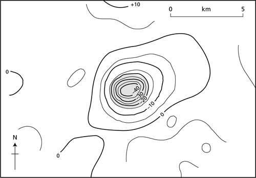
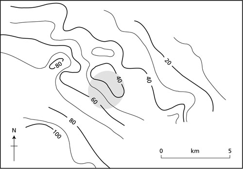
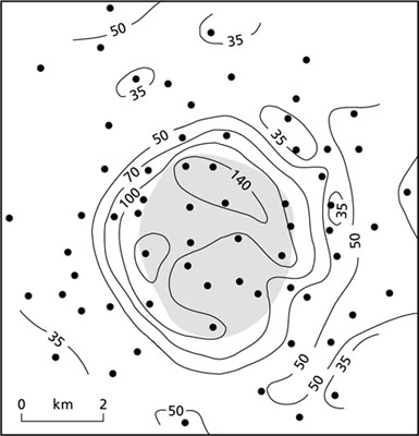
Fig. 1.2 Magnetic anomalies over the Grand Saline Salt Dome, Texas, USA (contours in nT — see Chapter 7). The stippled area represents the subcrop of the dome. (Redrawn from Peters & Dugan 1945.)
For a series of seismic rays travelling from a single shot point into a fan of seismic detectors (see Fig. 5.21), rays transmitted through any intervening salt dome will travel at a higher average velocity than in the surrounding medium and, hence, will arrive relatively early at the recording site. By means of this ‘fan-shooting’ it is possible to delineate sections of ground which are associated with anomalously short travel times and which may therefore be underlain by a salt body.
An alternative, and more effective, approach to the seismic location of salt domes utilizes energy reflected off the salt, as shown schematically in Fig. 1.3. A survey configuration of closely-spaced shots and detectors is moved systematically along a profile line and the travel times of rays reflected back from any subsurface geological interfaces are measured. If a salt dome is encountered, rays reflected off its top surface will delineate the shape of the concealed body.
Fig. 1.3 (a) Seismic reflection section across a buried salt dome (courtesy Prakla-Seismos GmbH). (b) Simple structural interpretation of the seismic section, illustrating some possible ray paths for reflected rays.
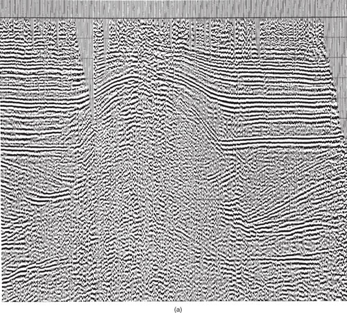
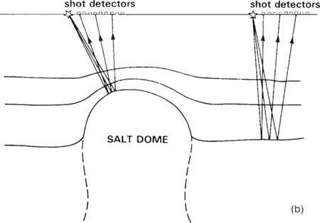
Fig. 1.4 Perturbation of telluric currents over the Haynesville Salt Dome, Texas, USA (for explanation of units see Chapter 9). The stippled area represents the subcrop of the dome. (Redrawn from Boissonas & Leonardon 1948.)
If the internal structure and physical properties of the Earth were precisely known, the magnitude of any particular geophysical measurement taken at the Earth’s surface could be predicted uniquely. Thus, for example, it would be possible to predict the travel time of a seismic wave reflected off any buried layer or to determine the value of the gravity or magnetic field at any surface location. In geophysical surveying the problem is the opposite of the above, namely, to deduce some aspect of the Earth’s internal structure on the basis of geophysical measurements taken at (or near to) the Earth’s surface. The former type of problem is known as a direct problem, the latter as an inverse problem. Whereas direct problems are theoretically capable of unambiguous solution, inverse problems suffer from an inherent ambiguity, or non-uniqueness, in the conclusions that can be drawn.
To exemplify this point a simple analogy to geophysical surveying may be considered. In echo-sounding, high-frequency acoustic pulses are transmitted by a transducer mounted on the hull of a ship and echoes returned from the sea bed are detected by the same transducer. The travel time of the echo is measured and converted into a water depth, multiplying the travel time by the velocity with which sound waves travel through water; that is, 1500 ms−1. Thus an echo time of 0.10 s indicates a path length of 0.10 × 1500 = 150 m, or a water depth of 150/2 = 75 m, since the pulse travels down to the sea bed and back up to the ship.
Using the same principle, a simple seismic survey may be used to determine the depth of a buried geological interface (e.g. the top of a limestone layer). This would involve generating a seismic pulse at the Earth’s surface and measuring the travel time of a pulse reflected back to the surface from the top of the limestone. However, the conversion of this travel time into a depth requires knowledge of the velocity with which the pulse travelled along the reflection path and, unlike the velocity of sound in water, this information is generally not known. If a velocity is assumed, a depth estimate can be derived but it represents only one of many possible solutions. And since rocks differ significantly in the velocity with which they propagate seismic waves, it is by no means a straightforward matter to translate the travel time of a seismic pulse into an accurate depth to the geological interface from which it was reflected.
The solution to this particular problem, as discussed in Chapter 4, is to measure the travel times of reflected pulses at several offset distances from a seismic source because the variation of travel time as a function of range provides information on the velocity distribution with depth. However, although the degree of uncertainty in geophysical interpretation can often be reduced to an acceptable level by the general expedient of taking additional (and in some cases different kinds of) field measurements, the problem of inherent ambiguity cannot be circumvented.
The general problem is that significant differences from an actual subsurface geological situation may give rise to insignificant, or immeasurably small, differences in the quantities actually measured during a geophysical survey. Thus, ambiguity arises because many different geological configurations could reproduce the observed measurements. This basic limitation results from the unavoidable fact that geophysical surveying attempts to solve a difficult inverse problem. It should also be noted that experimentally-derived quantities are never exactly determined and experimental error adds a further degree of indeterminacy to that caused by the incompleteness of the field data and the ambiguity associated with the inverse problem. Since a unique solution cannot, in general, be recovered from a set of field measurements, geophysical interpretation is concerned either to determine properties of the subsurface that all possible solutions share, or to introduce assumptions to restrict the number of admissible solutions (Parker 1977). In spite of these inherent problems, however, geophysical surveying is an invaluable tool for the investigation of subsurface geology and occupies a key role in exploration programmes for geological resources.
The above introductory sections illustrate in a simple way the very wide range of approaches to the geophysical investigation of the subsurface and warn of inherent limitations in geophysical interpretations.
Chapter 2 provides a short account of the more important data processing techniques of general applicability to geophysics. In Chapters 3 to 10 the individual survey methods are treated systematically in terms of their basic principles, survey procedures, interpretation techniques and major applications. Chapter 11 describes the application of these methods to specialized surveys undertaken in boreholes. All these chapters contain suggestions for further reading which provide a more extensive treatment of the material covered in this book. A set of problems is given for all the major geophysical methods.
Geophysical surveys measure the variation of some physical quantity, with respect either to position or to time. The quantity may, for example, be the strength of the Earth’s magnetic field along a profile across an igneous intrusion. It may be the motion of the ground surface as a function of time associated with the passage of seismic waves. In either case, the simplest way to present the data is to plot a graph (Fig. 2.1) showing the variation of the measured quantity with respect to distance or time as appropriate. The graph will show some more or less complex waveform shape, which will reflect physical variations in the underlying geology, superimposed on unwanted variations from non-geological features (such as the effect of electrical power cables in the magnetic example, or vibration from passing traffic for the seismic case), instrumental inaccuracy and data collection errors. The detailed shape of the waveform may be uncertain due to the difficulty in interpolating the curve between widely spaced stations. The geophysicist’s task is to separate the ‘signal’from the ‘noise’and interpret the signal in terms of ground structure.
Analysis of waveforms such as these represents an essential aspect of geophysical data processing and interpretation. The fundamental physics and mathematics of such analysis is not novel, most having been discovered in the 19th or early 20th centuries. The use of these ideas is also widespread in other technological areas such as radio, television, sound and video recording, radioastronomy, meteorology and medical imaging, as well as military applications such as radar, sonar and satellite imaging. Before the general availability of digital computing, the quantity of data and the complexity of the processing severely restricted the use of the known techniques. This no longer applies and nearly all the techniques described in this chapter may be implemented in standard computer spreadsheet programs.
The fundamental principles on which the various methods of data analysis are based are brought together in this chapter. These are accompanied by a discussion of the techniques of digital data processing by computer that are routinely used by geophysicists. Throughout this chapter, waveforms are referred to as functions of time, but all the principles discussed are equally applicable to functions of distance. In the latter case, frequency (number of waveform cycles per unit time) is replaced by spatial frequency or wavenumber (number of waveform cycles per unit distance).
Waveforms of geophysical interest are generally continuous (analogue) functions of time or distance. To apply the power of digital computers to the task of analysis, the data need to be expressed in digital form, whatever the form in which they were originally recorded.
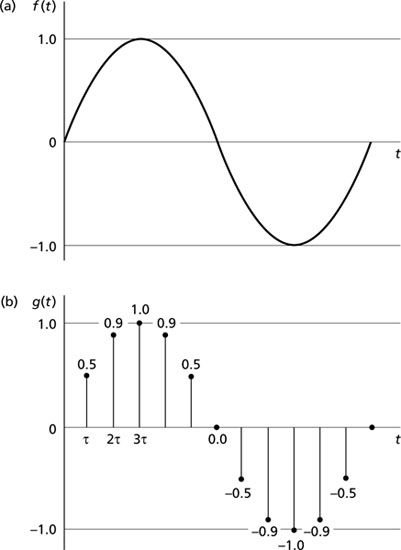
A continuous, smooth function of time or distance can be expressed digitally by sampling the function at a fixed interval and recording the instantaneous value of the function at each sampling point. Thus, the analogue function of time f(t) shown in Fig. 2.2(a) can be represented as the digital function g(t) shown in Fig. 2.2(b) in which the continuous function has been replaced by a series of discrete values at fixed, equal, intervals of time. This process is inherent in many geophysical surveys, where readings are taken of the value of some parameter (e.g. magnetic field strength) at points along survey lines. The extent to which the digital values faithfully represent the original waveform will depend on the accuracy of the amplitude measurement and the intervals between measured samples. Stated more formally, these two parameters of a digitizing system are the sampling precision (dynamic range) and the sampling frequency.
Dynamic range is an expression of the ratio of the largest measurable amplitude Amax to the smallest measurable amplitude Amin in a sampled function. The higher the dynamic range, the more faithfully the amplitude variations in the analogue waveform will be represented in the digitized version of the waveform. Dynamic range is normally expressed in the decibel (dB) scale used to define electrical power ratios: the ratio of two power values P1 and P2 is given by 10 log10(P1/P2) dB. Since power is proportional to the square of signal amplitude A
Fig. 2.1 (a) A graph showing a typical magnetic field strength variation which may be measured along a profile. (b) A graph of a typical seismogram, showing variation of particle velocities in the ground as a function of time during the passage of a seismic wave.
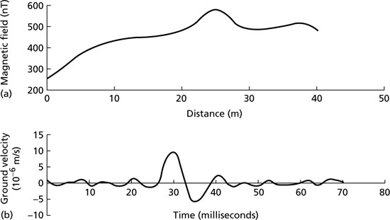
Fig. 2.2 (a) Analogue representation of a sinusoidal function. (b) Digital representation of the same function.
(2.1) 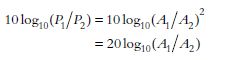
Thus, if a digital sampling scheme measures amplitudes over the range from 1 to 1024 units of amplitude, the dynamic range is given by

In digital computers, digital samples are expressed in binary form (i.e. they are composed of a sequence of digits that have the value of either 0 or 1). Each binary digit is known as a bit and the sequence of bits representing the sample value is known as a word. The number of bits in each word determines the dynamic range of a digitized waveform. For example, a dynamic range of 60dB requires 11-bit words since the appropriate amplitude ratio of 1024 (= 210) is rendered as 10000000000 in binary form. A dynamic range of 84 dB represents an amplitude ratio of 214 and, hence, requires sampling with 15-bit words. Thus, increasing the number of bits in each word in digital sampling increases the dynamic range of the digital function.
Sampling frequency is the number of sampling points in unit time or unit distance. Intuitively, it may appear that the digital sampling of a continuous function inevitably leads to a loss of information in the resultant digital function, since the latter is only specified by discrete values at a series of points. Again intuitively, there will be no significant loss of information content as long as the frequency of sampling is much higher than the highest frequency component in the sampled function. Mathematically, it can be proved that, if the waveform is a sine curve, this can always be reconstructed provided that there are a minimum of two samples per period of the sine wave.
Thus, if a waveform is sampled every two milliseconds (sampling interval), the sampling frequency is 500 samples per second (or 500 Hz). Sampling at this rate will preserve all frequencies up to 250 Hz in the sampled function. This frequency of half the sampling frequency is known as the Nyquist frequency (fN) and the Nyquist interval is the frequency range from zero up to fN
(2.2) 
where Δt = sampling interval.
If frequencies above the Nyquist frequency are present in the sampled function, a serious form of distortion results known as aliasing, in which the higher frequency components are ‘folded back’ into the Nyquist interval. Consider the example illustrated in Fig. 2.3 in which sine waves at different frequencies are sampled. The lower frequency wave (Fig. 2.3(a)) is accurately reproduced, but the higher frequency wave (Fig. 2.3(b), solid line) is rendered as a fictitious frequency, shown by the dashed line, within the Nyquist interval. The relationship between input and output frequencies in the case of a sampling frequency of 500 Hz is shown in Fig. 2.3(c). It is apparent that an input frequency of 125 Hz, for example, is retained in the output but that an input frequency of 625 Hz is folded back to be output at 125 Hz also.
To overcome the problem of aliasing, the sampling frequency must be at least twice as high as the highest frequency component present in the sampled function. If the function does contain frequencies above the Nyquist frequency determined by the sampling, it must be passed through an antialias filter prior to digitization. The antialias filter is a low-pass frequency filter with a sharp cut-off that removes frequency components above the Nyquist frequency, or attenuates them to an insignificant amplitude level.
An important mathematical distinction exists between periodic waveforms (Fig. 2.4(a)), that repeat themselves at a fixed time period T, and transient waveforms (Fig. 2.4(b)), that are non-repetitive. By means of the mathematical technique of Fourier analysis any periodic waveform, however complex, may be decomposed into a series of sine (or cosine) waves whose frequencies are integer multiples of the basic repetition frequency 1/T, known as the fundamental frequency. The higher frequency components, at frequencies of n/T (n = 1, 2, 3,…), are known as harmonics. The complex waveform of Fig. 2.5(a) is built up from the addition of the two individual sine wave components shown. To express any waveform in terms of its constituent sine wave components, it is necessary to define not only the frequency of each component but also its amplitude and phase. If in the above example the relative amplitude and phase relations of the individual sine waves are altered, summation can produce the quite different waveform illustrated in Fig. 2.5(b).
Fig. 2.3 (a) Sine wave frequency less than Nyquist frequency. (b) Sine wave frequency greater than Nyquist frequency (solid line) showing the fictitious frequency that is generated by aliasing (dashed line). (c) Relationship between input and output frequencies for a sampling frequency of 500 Hz (Nyquist frequency fN = 250 Hz).

Fig. 2.4 (a) Periodic and (b) transient waveforms.
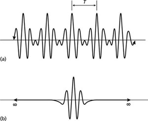
Fig. 2.5 Complex waveforms resulting from the summation of two sine wave components of frequency f and 2f. (a) The two sine wave components are of equal amplitude and in phase. (b) The higher frequency component has twice the amplitude of the lower frequency component and is π/2 out of phase. (After Anstey 1965.)

Fig. 2.6 Representation in the frequency domain of the waveforms illustrated in Fig. 2.5, showing their amplitude and phase spectra.

From the above it follows that a periodic waveform can be expressed in two different ways: in the familiar time domain, expressing wave amplitude as a function of time, or in the frequency domain, expressing the amplitude and phase of its constituent sine waves as a function of frequency. The waveforms shown in Fig. 2.5(a) and (b) are represented in Fig. 2.6(a) and (b) in terms of their amplitude and phase spectra. These spectra, known as line spectra, are composed of a series of discrete values of the amplitude and phase components of the waveform at set frequency values distributed between 0 Hz and the Nyquist frequency.
Transient waveforms do not repeat themselves; that is, they have an infinitely long period. They may be regarded, by analogy with a periodic waveform, as having an infinitesimally small fundamental frequency (1/T → 0) and, consequently, harmonics that occur at infinitesimally small frequency intervals to give continuous amplitude and phase spectra rather than the line spectra of periodic waveforms. However, it is impossible to cope analytically with a spectrum containing an infinite number of sine wave components. Digitization of the waveform in the time domain (Section 2.2) provides a means of dealing with the continuous spectra of transient waveforms. A digitally sampled transient waveform has its amplitude and phase spectra subdivided into a number of thin frequency slices, with each slice having a frequency equal to the mean frequency of the slice and an amplitude and phase proportional to the area of the slice of the appropriate spectrum (Fig. 2.7). This digital expression of a continuous spectrum in terms of a finite number of discrete frequency components provides an approximate representation in the frequency domain of a transient waveform in the time domain. Increasing the sampling frequency in the time domain not only improves the time-domain representation of the waveform, but also increases the number of frequency slices in the frequency domain and improves the accuracy of the approximation here too.
Fig. 2.7 Digital representation of the continuous amplitude and phase spectra associated with a transient waveform.

Fourier transformation may be used to convert a time function g(t) into its equivalent amplitude and phase spectra A(f) and ϕ(f), or into a complex function of frequency G(f) known as the frequency spectrum, where
(2.3) 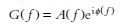
The time- and frequency-domain representations of a waveform, g(t) and G(f), are known as a Fourier pair, represented by the notation
(2.4) 
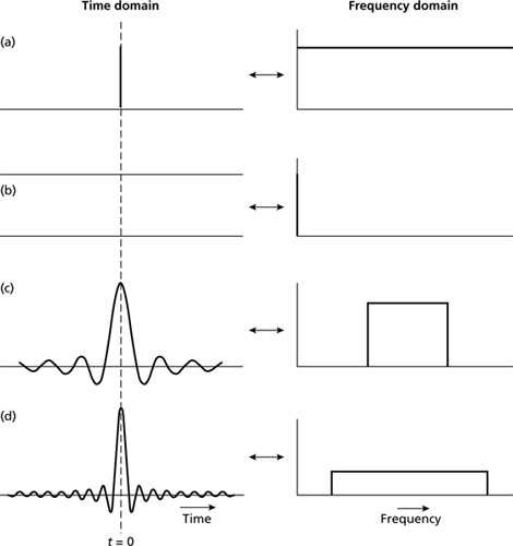
Components of a Fourier pair are interchangeable, such that, if G(f) is the Fourier transform of g(t), then g(t) is the Fourier transform of G(f). Figure 2.8 illustrates Fourier pairs for various waveforms of geophysical significance. All the examples illustrated have zero phase spectra; that is, the individual sine wave components of the waveforms are in phase at zero time. In this case ϕ(f) = 0 for all values of ϕ. Figure 2.8(a) shows a spike function (also known as a Dirac function), which is the shortest possible transient waveform. Fourier transformation shows that the spike function has a continuous frequency spectrum of constant amplitude from zero to infinity; thus, a spike function contains all frequencies from zero to infinity at equal amplitude. The ‘DC bias’ waveform of Fig. 2.8(b) has, as would be expected, a line spectrum comprising a single component at zero frequency. Note that Fig. 2.8(a) and (b) demonstrate the principle of interchangeability of Fourier pairs stated above (equation (2.4)). Figures 2.8(c) and (d) illustrate transient waveforms approximating the shape of seismic pulses, together with their amplitude spectra. Both have a bandlimited amplitude spectrum, the spectrum of narrower bandwidth being associated with the longer transient waveform. In general, the shorter a time pulse the wider is its frequency bandwidth and in the limiting case a spike pulse has an infinite bandwidth.
Waveforms with zero phase spectra such as those illustrated in Fig. 2.8 are symmetrical about the time axis and, for any given amplitude spectrum, produce the maximum peak amplitude in the resultant waveform. If phase varies linearly with frequency, the waveform remains unchanged in shape but is displaced in time; if the phase variation with frequency is non-linear the shape of the waveform is altered. A particularly important case in seismic data processing is the phase spectrum associated with minimum delay in which there is a maximum concentration of energy at the front end of the waveform. Analysis of seismic pulses sometimes assumes that they exhibit minimum delay (see Chapter 4).
Fourier transformation of digitized waveforms is readily programmed for computers, using a ‘fast Fourier transform’ (FFT) algorithm as in the Cooley–Tukey method (Brigham 1974). FFT subroutines can thus be routinely built into data processing programs in order to carry out spectral analysis of geophysical waveforms. Fourier transformation is supplied as a function to standard spreadsheets such as Microsoft Excel. Fourier transformation can be extended into two dimensions (Rayner 1971), and can thus be applied to areal distributions of data such as gravity and magnetic contour maps. In this case, the time variable is replaced by horizontal distance and the frequency variable by wavenumber (number of waveform cycles per unit distance). The application of two-dimensional Fourier techniques to the interpretation of potential field data is discussed in Chapters 6 and 7.
Fig. 2.8 Fourier transform pairs for various waveforms. (a) A spike function. (b) A ‘DC bias’. (c) and (d) Transient waveforms approximating seismic pulses.
The principles of convolution, deconvolution and correlation form the common basis for many methods of geophysical data processing, especially in the field of seismic reflection surveying. They are introduced here in general terms and are referred to extensively in later chapters. Their importance is that they quantitatively describe how a waveform is affected by a filter. Filtering modifies a waveform by discriminating between its constituent sine wave components to alter their relative amplitudes or phase relations, or both. Most audio systems are provided with simple filters to cut down on highfrequency ‘hiss’, or to emphasize the low-frequency ‘bass’. Filtering is an inherent characteristic of any system through which a signal is transmitted.
Convolution (Kanasewich 1981) is a mathematical operation defining the change of shape of a waveform resulting from its passage through a filter. Thus, for example, a seismic pulse generated by an explosion is altered in shape by filtering effects, both in the ground and in the recording system, so that the seismogram (the filtered output) differs significantly from the initial seismic pulse (the input).
As a simple example of filtering, consider a weight suspended from the end of a vertical spring. If the top of the spring is perturbed by a sharp up-and-down movement (the input), the motion of the weight (the filtered output) is a series of damped oscillations out of phase with the initial perturbation (Fig. 2.9).
The effect of a filter may be categorized by its impulse response which is defined as the output of the filter when the input is a spike function (Fig. 2.10). The impulse response is a waveform in the time domain, but may be transformed into the frequency domain as for any other waveform. The Fourier transform of the impulse response is known as the transfer function and this specifies the amplitude and phase response of the filter, thus defining its operation completely. The effect of a filter is described mathematically by a convolution operation such that, if the input signal g(t) to the filter is convolved with the impulse response f(t) of the filter, known as the convolution operator, the filtered output y(t) is obtained:
(2.5) 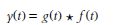
where the asterisk denotes the convolution operation.
Fig. 2.9 The principle of filtering illustrated by the perturbation of a suspended weight system.
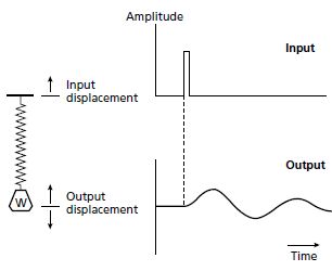
Figure 2.11(a) shows a spike function input to a filter whose impulse response is given in Fig. 2.11(b). Clearly the latter is also the filtered output since, by definition, the impulse response represents the output for a spike input. Figure 2.11(c) shows an input comprising two separate spike functions and the filtered output (Fig. 2.11(d)) is now the superposition of the two impulse response functions offset in time by the separation of the input spikes and scaled according to the individual spike amplitudes. Since any transient wave can be represented as a series of spike functions (Fig. 2.11(e)), the general form of a filtered output (Fig. 2.11(f)) can be regarded as the summation of a set of impulse responses related to a succession of spikes simulating the overall shape of the input wave.
giimf( = 1, 2, . . . , ) is a convolution operator, then the convolution output function k